9. Field

Guide to conducting field surveys using open-source tools

9.1. Background

Using field surveys to create geospatial data is a common practice but can require costly hardware, subscriptions for cloud data, and syncing. I’ve found that QField, which syncs with QGIS, could be great, but the forms are clunky, and the cloud setup is not easy. I got it to work, but I wouldn’t say I liked entering the data. ESRI’s Survey 123 is a paid software, part of a subscription to Arc or other software. It is very easy to set up and sync data, plus you have instant maps of recorded data in the field. Survey 123 was the quickest to pinpoint GPS location. It comes at a cost, but it may be worth it if you do a lot of field surveys. The data is accessible after you send it in the Portal tab of the catalog window. Very seamless.

Even if you conduct many surveys, the Kobo Toolbox is brilliant. Survey forms are easy to set up and sync to your phone, and filling them out in the field is easy. Plus, there is no limit to storing data or pricing, which is a huge plus. Kobo is used by many humanitarian organizations worldwide throughout crises, so the software developers here have made it very easy to use.

9.2. Quick start

1. Sign up for an account at Kobo Toolbox. Download KoboCollect to your phone and sign in.

2. Open the forms and add questions in the Kobo toolbox, then Deploy once it’s ready.

3. Sync the survey to your phone (Download form) and ensure it’s uploaded and working.

4. In the field, open the Kobo app, click + Start new form and enter the data.

5. When finished collecting, go to Ready to send, select all, and send.

6. Back at your online Kobo account, click the data tab, and all the forms you filled out will be there.

7. Download the data in Excel, csv, or geojson. I found the Excel download best, then converted that file to csv after modifying unnecessary columns. Note that you don’t need to add date, unique field, or time as fields to the form since they are automatically added.

8. Import the csv into a notebook, QGIS, or Kepler to view it.

9.3. Stand Density Index

Foresters have long used stand density index (SDI) to measure forest stocking levels since it is calculated from size and number of trees per unit area [Reineke, 1933]. Since it also measures inter-specific tree competition and how crowded a stand is [North et al., 2022] used it as a proxy estimate for forest health using the summation method:

\[ \sum TPH_i\left( \frac{DBH_i}{25.4}\right)^{\!1.6} \]

where TPH = trees ha^-1 of tree_i and DBH_i = diameter breast height (cm) of tree_i.

The summation method is recommended for uneven-age or irregular structure stands [Shaw, 2000]. It is appropriate to stands found in the New Forest, a mixture of non-native plantation species such as Scot Pine (Pinus sylvestris) and Douglas fir (Pseudotsuga menziesii) with native species such as English Oak (Quercus robur), beech (Fagus sylvatica), and holly (Ilex aquifolium).

9.4. Methodology

To examine forest health in a local forest stand, I measured trees > 30 cm in dbh circumference within 500 m² plots at the forested areas randomly sampled from the New Forest National Park, United Kingdom. The sample data shown is from the first three measured plots at Norleywood Enclosure.

9.5. Field data

Fig. 9.1 shows the Kobo Collect start screens. Before you travel to the field, click Download Form to upload the survey to your phone.

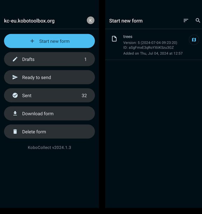
Fig. 9.1 Kobo Collect start screens.

Click + Start new form at the top of the screen, and click on the survey name, which brings up the first data entry point. In this case, it’s the location screen shown in Fig. 9.2.

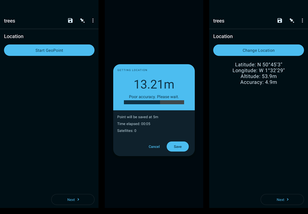
Fig. 9.2 Location screens.

Click Start GeoPoint. The app will start searching for location and give you a confirmation once it gets to 5m or less as shown in the right two screenshots of Fig. 9.2. It may take a few seconds. If it’s taking some time, you may need to point the phone towards the open sky. Click next and proceed to the remainder of the data entry (Fig. 9.3).

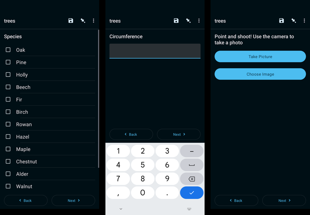
Fig. 9.3 Survey form screens.

It is worth keeping questions and answers brief in each section. Note that I just put short common names for tree species in the order of their abundance to make filling out the species section easier. Once you’ve completed the forms, you’ll be prompted to finalize and send. (Fig. 9.4)

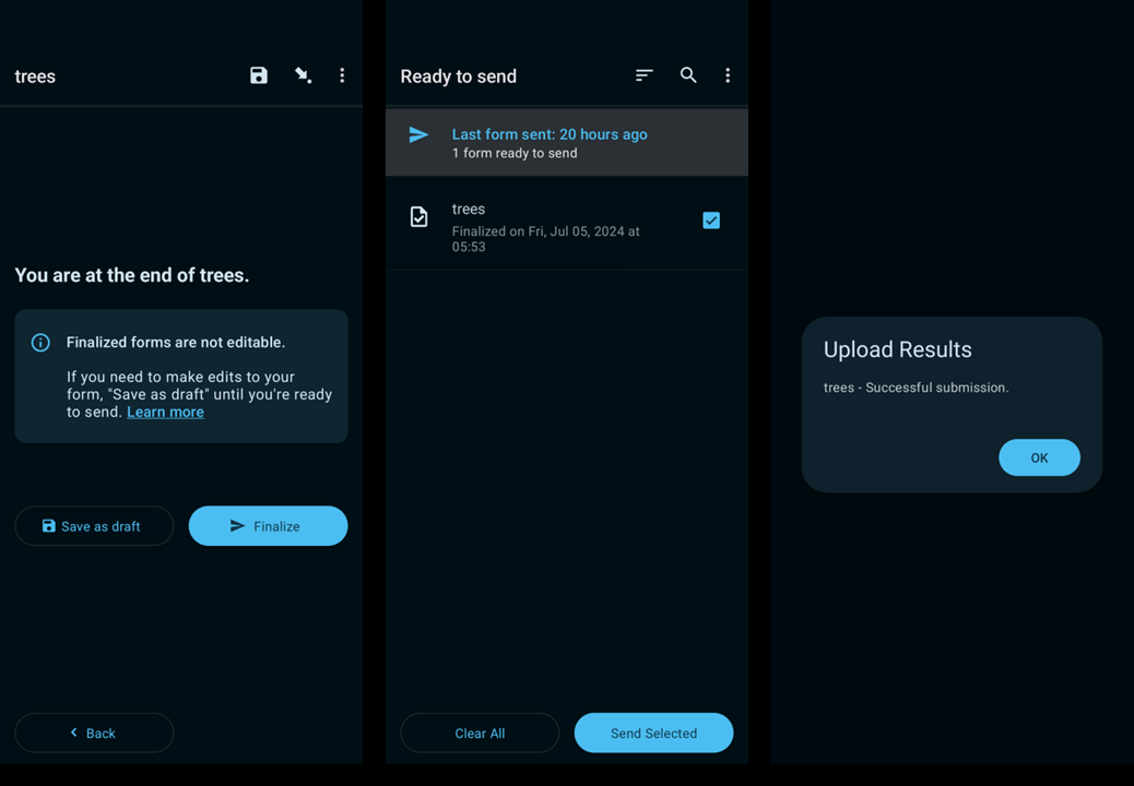
Fig. 9.4 Send screens.

After completing each survey, you’ll be returned to the home screen. Once finished with the site or the day’s entries, click Ready to send, Select All (at the bottom left), and Send Selected. You’ll get an Upload Results/Successful submission message.

Back in the Kobo Toolbox online, click on Data table where you’ll be able to view, sort, and edit everything you collected as shown in Fig. 9.5.

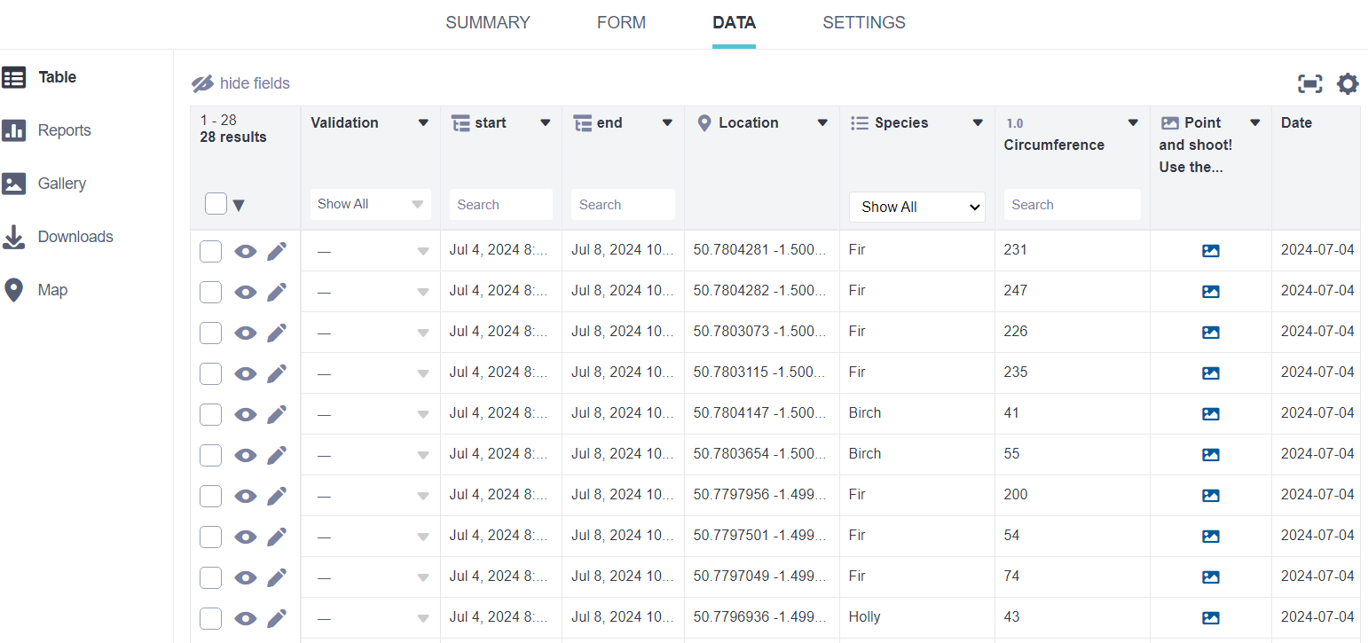
Fig. 9.5 KoboToolbox Data/Table tab.

If you select the Reports tab, you’ll get descriptive statistics for each survey question. Although this section allows you to create custom reports, it doesn’t let you change information, axes, or build in any analysis, but it’s still pretty useful for an at-a-glance of your data (Fig. 9.6).

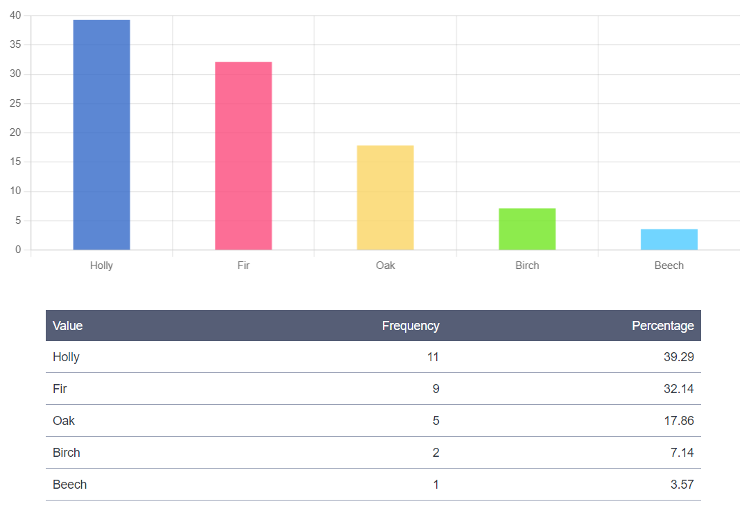
Fig. 9.6 KoboToolbox Data/Report tab.

Clicking the Gallery gives you all of the photos you took sequentially. You can download and save each one by clicking on the photo. Look at those beautiful tree trunks in the forest (Fig. 9.7).

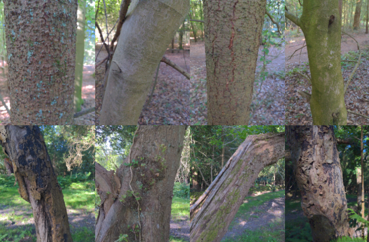
Fig. 9.7 KoboToolbox Data/Gallery tab.

The Downloads tab does ‘exactly what it says on the tin’, as some English folks are wont to say. I downloaded the data first as an Excel sheet, edited it, and then saved it as a CSV that’s in the repo under the file /test/norley2.csv. Make sure you change the lat/lon columns to a clear name, such as Latitude or longitude, to make them easier to pick up with the software you use.

9.6. Visualization

I didn’t completely figure out the geojson download. It was a bit clunky because it converted the data to geojson and opened it in a web browser instead of downloading it as a geojson file. The coding looked correct, however.

You can then upload and analyze data using Python libraries, QGIS, or other software. If you add via QGIS:

1. Click on the Data Source Manager (or control/command L, or Layer/Add Layer/Add Delimited Text Layer). Make sure the Delimited Text tab to the left is selected. Latitude and Longitude should be recognized in the Point coordinate section. Make sure that X is longitude and Y is latitude.

2. Click the three dots next to the File name and navigate to where the csv file is stored.

3. Name the layer under the Layer name.

4. At the Geometry CRS, ensure the imported table is the same Coordinate Reference System as the QGIS project.

5. You should see a sample table at the bottom. Click add, and the points should be added to the project. If you don’t see them where they’re supposed to be or they ended up in West Africa, you need to reconcile the projections.

Let’s look at a simpler/nearly instantaneous way to view and stylize the points. Make sure you have the Geo Data Viewer installed in Visual Studio Code. Right-click on the norley2.csv and select View Map. This brings up the dataset using kepler.gl. It looks pretty good right away. Here are a couple of quick changes:

1. Click the down arrow on the point layer to expand it. Reduce the Radius of the points to see them more clearly.

2. Click the three buttons next to Fill Color, and in Color Based On, replace the default value with Species or Diameter. You can also change the coloramp here. Color based on circumference gives you a visual of the size distribution.

3. The Label value lets you select any field to add a label to each point.

Fig. 9.8 shows a rather handsome map that can add additional layers and change or customize the symbology.

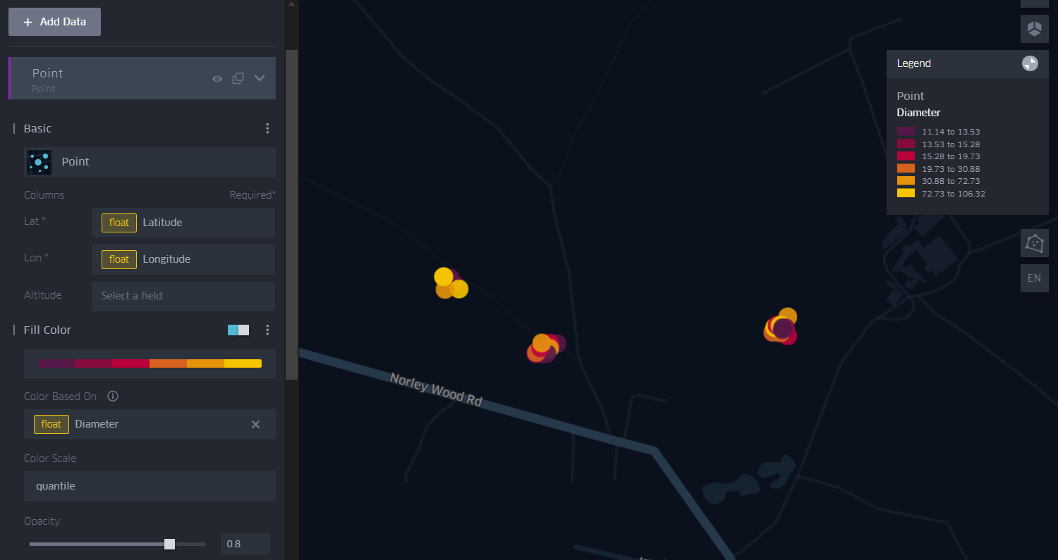
Fig. 9.8 The kepler.gl map of the points using Geo Data Viewer and Visual Studio Code.

9.7. SDI

The total number of trees sampled for the size stand is not sufficient, but with the figures in hand, the SDI estimate would be approximately 123. Sampling additional stands across the New Forest and comparing them to historical National Forest Inventory values will better indicate this stand’s comparative health.

There’s your start from collection to visualization. Hopefully, this will inspire you to collect some needed data for your organization, agency, or dissertation! Additional resources are provided below.

9.8. Resources

• Kobo Toolbox. An open-source data collection platform that’s easy to use and set up. Kobo is a form-based app that syncs to the cloud so you need to export the csv or geojson files and then load them into your geospatial analysis software of choice.

• ODK. Free if you can self-host and support.

• QField. Survey and digitize data mobile app that syncs to QGIS. The QField setup tutorial from GISGeography runs you through the basics to get up and running. QField would be amazing if it were easy to set up and use. Unfortunately, its use is more difficult than anticipated. The cloud sync works but does not allow much storage. You can pay for increased storage, however. It’s a great idea, but it needs a lot more work to be easier.