4. Python

Python is widely applicable and used in the geospatial community. ArcGIS Pro has a Python package called Arcpy, and QGIS has a package named PYQGIS. It could be me, but I tried using Arcpy, read through and tried the tutorials from an entire Arcpy book, and struggled using ESRI notebooks. The language didn’t stick with me, and it was overly complicated. Sure, you could run an analysis tool and copy the Arcpy code into a notebook to modify it, but I had a ‘block’ developing code blocks.

Then I found Geemap and Leafmap—incredible, user-friendly Python packages developed by Qiusheng Wu and available on GitHub at GISWQS. There are also clear tutorials at leafmap.org and geemap.org and videos at Open Geospatial Solutions. Many analyses require only one line of code. Here, geospatial analysis using scripts just clicked for me, opening up another world to analyze geospatial data.

4.1. Getting Started

To be honest, getting started using a Windows computer was a total pain in the ass. So, if you’re using Linux or Apple OS, setting things up will be much easier. It will take a few hours from scratch, but a great resource is at the Geog-414 course software web page. Scroll through the page to familiarize yourself with the commands. Near the bottom of the page is a series of videos to get you started, which is worth viewing and following. For some reason, I found that Miniconda didn’t work well on my machine with Windows 11, but everything worked with Anaconda.

Important

Getting started quick guides can be found in the Virtual Environment, Visual Studio Code, and Github appendices.

To get you up and running quickly, I’ve provided a cheat sheet in the Virtual Environment appendix that summarizes the Geog-414 videos and should have you started quickly. However, you may want to refer to the videos if you get stuck.

4.2. Sentinel-2 Data

Before you do that, let’s look at a simple example from a GitHub gist posted by Alex Leith. We’ll run it in Colab. Click the Open in Colab button.

Google Colab is an online notebook that lets you write and execute code. Its advantage is that it is shareable, connected to your Google account, and performs calculations in the cloud. The disadvantage is once you close the notebook, everything you’ve installed or executed will disappear, although the code is saved. It’s great for quickly testing out Python script in a notebook environment.

Note

‘Uncommenting’ a line in Python means removing the hashtag before the command or clicking on the line, then clicking control or command plus backslash (/).

Install the dependencies:

# Uncomment the line below to install pystac and odc
# !pip install pystac-client odc-stac odc-geo

and import

# Import dependencies
from pystac_client import Client
from odc.stac import load
import odc.geo.xr

Access data and create a bounding box:

# Earth search provides access to a wide range of data sources
client = Client.open("https://earth-search.aws.element84.com/v1")
collection = "sentinel-2-l2a"

# Create a bounding box centered in Tasmania
# The bounding box is lower-left x, lower-left y, upper-right x, upper-right y
bbox = [146.5, -43.6, 146.7, -43.4]

Hint

Use Earth Engine’s inspector or the polyline tool to generate coordinates.

Search and load the data:

# Datetime can be a single date, YEAR, YEAR-MONTH or YEAR-MONTH-DAY
# or a range, YEAR-MONTH/YEAR-MONTH
datetime = "2023-12"

# Run a lazy-loaded search of the STAC API
search = client.search(collections=[collection], bbox=bbox, datetime=datetime)

# Pass the search results to the load function, which will lazy-load the data
data = load(search.items(), bbox=bbox, groupby="solar_day", chunks={}, crs="EPSG:8857", resolution=10)

The search.items() part of the data variable threw an error when running this codeblock in VS Code. However, it works in Colab.

Visualize it:

# Visualize the data
# Time=2 is an arbitrary time slice picked because there's few clouds
data[["red", "green", "blue"]].isel(time=2).to_array().plot.imshow(vmin=0, vmax=1500)

# Alternately, you could visualise using odc.geo.xr's explore function
# data.isel(time=2).explore(bands=["red", "green", "blue"], vmin=0, vmax=1500)

Fig. 4.1 shows the resulting Sentinel-2 true color image.

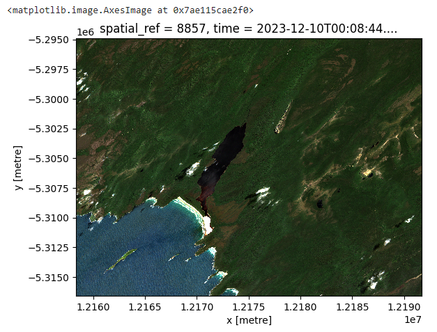
Fig. 4.1 True color Sentinel-2 image.

The access and sharing of this code are another example of why free and open-source software is special. The community is willing to share it, and it is reproducible and easily modified to meet your needs.

4.3. Geemap

Compared to Javascript, Geemap is a much easier way to access, analyze, and visualize Earth Engine data, all within a Python package environment developed by Qiusheng Wu.

Getting Started

Watch this installation video followed by this vs code and github video. If you already have an IDE, Miniconda, and virtual env’s installed, go to the Geemap installation page.

Let’s look at how to visualize the same map from Chapter 2 using Geemap. Open a Jupyter notebook and add the following code block:

# Import geemap and create an interactive map
import ee
import geemap
geemap.ee_initialize()
m = geemap.Map()
m

To give you a generic world map with map widgets (Fig. 4.2).

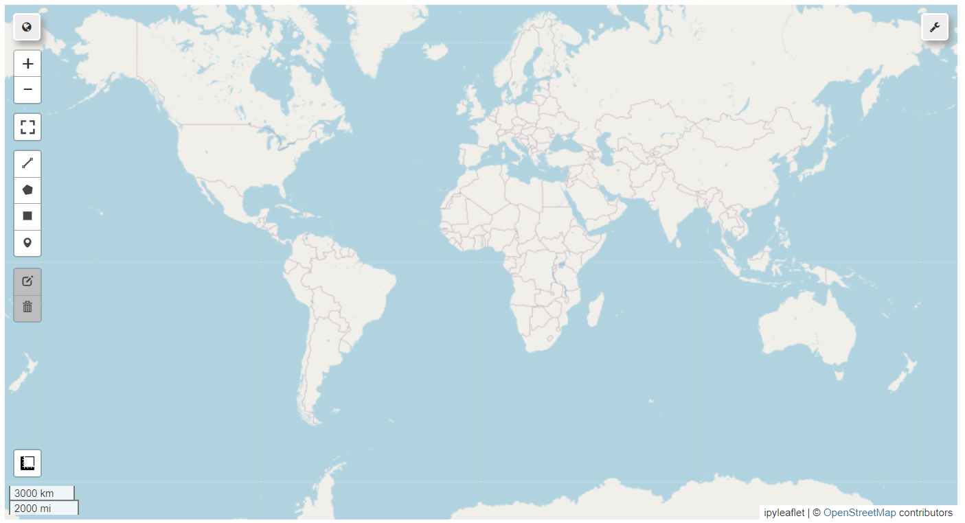
Fig. 4.2 Interactive map in Geemap.

In the upper right corner of the map, click the wrench icon, then click the two encircling arrows box (bottom row, middle) to open the Javascript to Python code converter (Fig. 4.3).

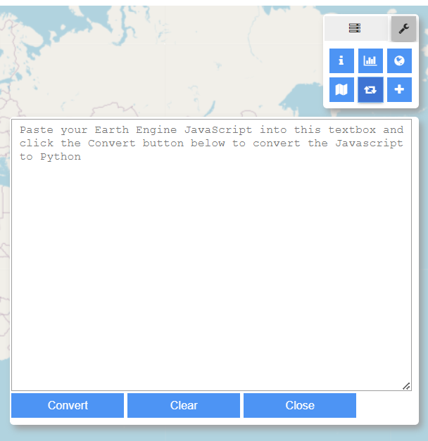
Fig. 4.3 Textbox converter for Earth Engine Javascript to Python.

Go to the Earth Engine code editor, open the script from Chapter 2, select all, and paste it into the converter. Click the convert button. The code is copied to the clipboard. Paste it into a new code block and comment out the definition function on lines 4-6:

# Add global carbon density map
dataset = ee.ImageCollection('NASA/ORNL/biomass_carbon_density/v1')

# def func_rif(image)return image.clip(bbox)};: \
#                     .map(function(image){return image.clip(bbox)} \
#                     .map(func_rif)

# Add visual parameter variables
vis_a = {
  'bands': ['agb'],
  'min': -50.0,
  'max': 80.0,
  'palette': ['d9f0a3', 'addd8e', '78c679', '41ab5d', '238443', '005a32']
}

vis_b = {
  'bands': ['bgb'],
  'min': -50.0,
  'max': 80.0,
  'palette': ['D6BCB1', 'AB8574', '784E3D', '3D2216', '26140C', '000000']
}

# Center map and add layers
m.setCenter(-120.2348, 38.8744, 9)
m.addLayer(dataset, vis_a, 'Aboveground biomass carbon')
m.addLayer(dataset, vis_b, 'Belowground biomass carbon')
m

Running that code block will result in Fig. 4.4.

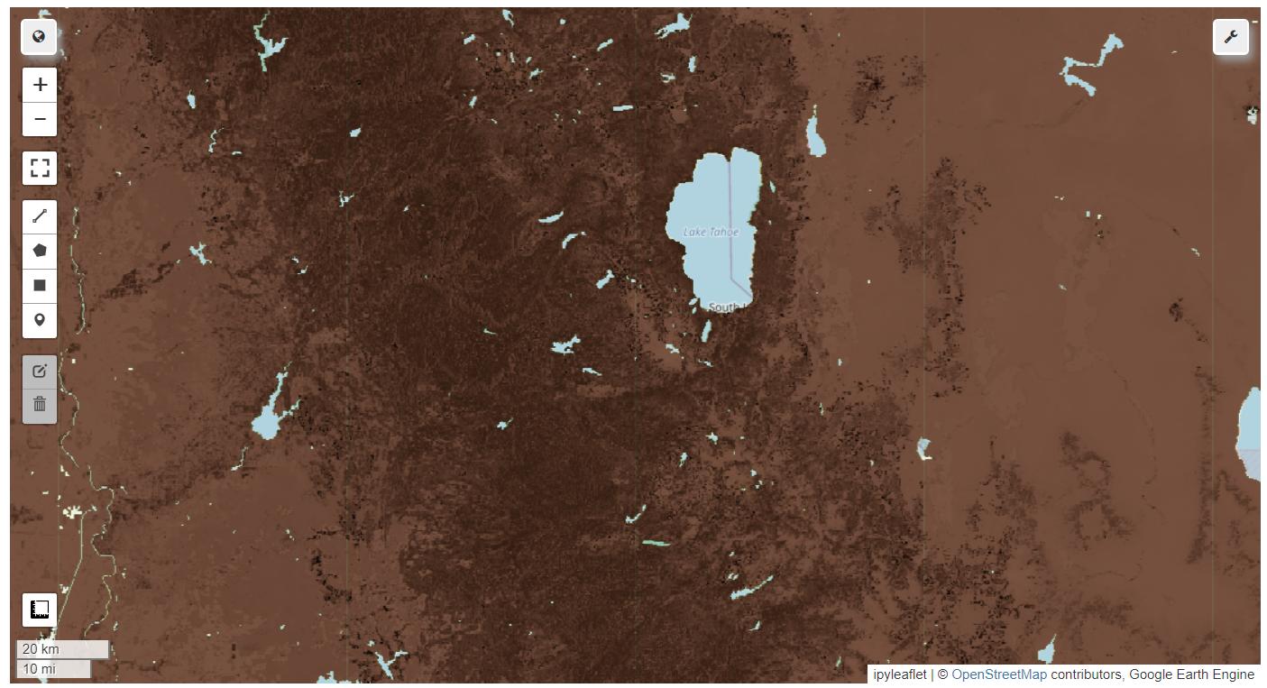
Fig. 4.4 Adding above and belowground biomass carbon with belowground showing.

If you return to the wrench icon and select the layers icon to the left, you can switch layers on and off (Fig. 6.3).

Fig. 4.5 Layers panel.

Add a new code block and add an area of interest called bbox, short for bounding box:

Tip

To run the code in a code block, click ctrl/command + enter. To run the code and add a new code block, click alt + enter.

# Add an area of interest
bbox = [-121.1874, 38.2931, -119.5262, 39.2884]
bbox = ee.Geometry.Rectangle(bbox)

Then clip the carbon raster to the AOI:

# Clip the dataset to the area of interest
aoi = dataset.map(lambda image: image.clip(bbox))

Now add the clipped rasters:

# Add the clipped dataset to the map
m.addLayer(aoi, vis_b, 'AOI belowground biomass carbon')
m.addLayer(aoi, vis_a, 'AOI aboveground biomass carbon')
m

If you turn off the aboveground and belowground maps, a map with the clipped aboveground biomass carbon layer will result (Fig. 4.6).

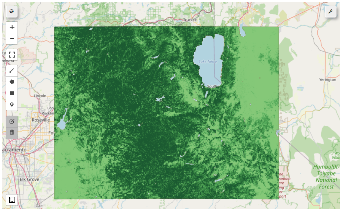
Fig. 4.6 Raster clipped to area of interest with aboveground biomass carbon visible.

Delete the function from the javascript conversion that you commented out previously in lines 4-6. If you need to keep running and test the map, you can turn off the original biomass layers added for the entire globe by changing the center map add map layers to the code block to

# Center map and add layers
m.setCenter(-120.2348, 38.8744, 9)
m.addLayer(dataset, vis_a, 'Aboveground biomass carbon', False)
m.addLayer(dataset, vis_b, 'Belowground biomass carbon', False)

Adding ‘False’ after the layer name still adds the layers to the map but turns them off by default.

Lambda Function

Let’s take another look at the lambda function to clip the raster. Lambda functions are similar to other Python functions but are not bound to a name when run. Known as anonymous functions, they are used when you need a one-off function that isn’t separately defined. In our case, the Lamda function takes an image, clips it to the bounding box, and returns the clipped image. The map() function, not to be confused with the Map function in Javascript, applies the function to every image in the ImageCollection.

4.4. Easier bboxing

Boots and cats, boots and cats, boots and cats. Yeah! No wait, it’s bounding boxing, not beat boxing! As you can see in both examples, adding the code for a bounding box can be semi-painful. The Polyline Tool allows you to create the needed code when you right-click each point in a polygon.

# Import geemap and initialize earth engine
import ee
import geemap
geemap.ee_initialize()
m = geemap.Map()

In the Polyline Tool, I’ve right-clicked 3 points around Cape Cod, Massachusetts, in the United States, then clicked close shape to get a square. Then, I copied the curly brackets and the geojson coordinates in between and assigned them to a variable. Then, convert the geojson coordinates to an earth engine geometry type and map.

# Add the coordinates from the Polyline tool and assign to a variable
capecod = {
    "coordinates": [
        [
            [
                -70.4525757,
                42.0916883
            ],
            [
                -70.423462,
                41.4974371
            ],
            [
                -69.7763673,
                41.5036664
            ],
            [
                -69.7939453,
                42.1075947
            ],
            [
                -70.4525757,
                42.0916883
            ]
        ]
    ],
    "type": "Polygon"
}

# Convert the geojson coordinates to ee.Geometry and map
bbox = ee.Geometry(capecod)
m.addLayer(bbox, {}, 'Cape Cod')
m

You may need to zoom into Cape Cod to see the box. This somewhat lengthy method allows you to create any global polygon with as many points as you like.

4.5. Leafmap

A related Python package worth exploring is Leafmap, also developed by Qiusheng Wu and focused on geospatial data analysis and visualization. Leafmap is increasing its 3d capabilities, great for terrain and building visualization. Like Geemap, the site has extensive documentation and tutorials. I highly recommend attending one of the Leafmap workshops, which will guide you through installation, examples, and many use cases.

Notebooks and videos support the tutorials and workshops to walk you through this excellent software package. Click on the links provided to run the code in Binder or Colab. If you wanted to run a workshop in VS Code:

1. Click workshops in leafmap.org

2. Select the workshop

3. Select GitHub in the upper right, select examples, then notebooks

4. Click on the notebook you want (*.ipynb)

5. Below history in the upper right of your browser, click on the download raw file button, save the file, and then click to open it in VS Code.

6. Alternatively, go straight to the workshop notebooks, such as the FOSS4G Workshop.

Before running the code cells, ensure Leafmap is installed in your environment. For a quick starter guide on how to do this, see the miniconda/anaconda section of the FOSS4G workshop.

There are many more Python libraries focused on geospatial analysis. Go to github.com and search for them or find them through online tutorials, medium.com, X (Twitter), and LinkedIn. Below are some additional resources to help you go deeper.

4.6. Resources

• Geemap has a webpage, book, tutorials, API, and much more to support this excellent Python package.

• Leafmap is a Python package for geospatial analysis in a Jupyter environment. It has superb documentation, tutorials, and ease of use.

• Open Geospatial Solutions hosts many open-source geospatial software projects and datasets. Spatial Thoughts, run by Ujaval Gandhi, offers a free course called Python Foundation for Spatial Analysis. The site also provides many other free and paid courses and tutorials for geospatial analysis.

• Geocomputation with Python is an open source book inspired by the FOSS4G movement.

• RiverREM. A super cool Python package for automatically generating river relative elevation model (REM).

• lonboard. Python library for fast geospatial vector data visualization.

• Python for Ecologists. The Datacarpentry.org tutorial focused on data analysis and visualization using Python and Jupyter notebooks. This is more data than geospatial, but it is a useful set of tutorials.

• Unlocking the Depths. A useful tutorial for mapping bathymetry and calculating lake volume, although it may be behind a paywall.