SQL

5. SQL#

The language to learn for geospatial analysis!

5.1. New#

SQL is pronounced ‘sequel’ and is short for structure query language. I’m new to using SQL for geospatial analysis. Still, I am amazed at how easy it is to learn, how fast it analyzes large datasets, and how critical it is for data analysis. SQL is the universal database management language, so geospatial aside, if you work with data, you must learn how to use it. The basic structure of a SQL query is shown in the tips window. Initially, the CREATE and SELECT * FROM commands are used in data exploration, followed by finer-scale querying.

Tip

BASIC SQL QUERY STRUCTURE
CREATE TABLE IF NOT EXISTS tablename AS
SELECT * FROM (‘path_to_file’)
WHERE
GROUP BY
ORDER BY desc
LIMIT

5.2. DuckDB#

In this chapter, we will use DuckDB as the SQL software package. DuckDB is fast, works seamlessly with many programming languages, including Python, R, and Javascript, and is easy to install. DuckDB also has a spatial extension to perform queries and analyze geospatial data, which we will look at in this chapter. The big advantage of DuckDB is its speed in processing large datasets.

5.3. Installation#

Installation is straightforward: follow the instructions for the command line or Python at the DuckDB installation page.

5.4. Wood processing#

Let’s move to an example from the University of California’s Woody Biomass Utilization Group’s Biomass Power Plant Database. What do mills have to do with forest conservation? We’re not talking about rapacious clearcutting from the past but a sustainable forest management model that reduces wildfire and returns western forests to a healthier and more resilient state. Fires threaten most forests in the western United States due to more than a century of fire suppression.

Through ecological thinning and prescribed fire, unhealthy forests can return to a natural range of variation by lowering competition across stands. This approach can reduce compounding stresses from drought, insect infestations, and wildfire and create more resilient forests [North et al., 2022]. Thinning will produce large amounts of forest biomass that can be processed through community-based mills and biomass plants. Developing this infrastructure is one way to help solve the wildfire crisis threatening biodiversity and people.

First, import the dependencies.

# import dependencies
import duckdb
import leafmap
import pandas as pd

Then, connect to the duckdb database and install httpfs and spatial extensions.

# Connect database install httpfs, spatial
con = duckdb.connect()
con.install_extension("httpfs")
con.load_extension("httpfs")
con.install_extension("spatial")
con.load_extension("spatial")

Read the sawmill .shp file and create the sawmill table.

# Create sawmill table from shp file and show table
con.sql('''
    CREATE TABLE IF NOT EXISTS sawmill as
    SELECT * FROM ST_Read('./wood.shp')
''')
con.table('sawmill')

Note that ./ reads the sawmill shape file in the CurrentSawmill file if you’ve cloned the repo to your local computer. If you downloaded a shp file in Windows to your Downloads folder, replace the path to where you’ve stored the shp files, for example, ‘C:/Users/your_user_name/Downloads/shapefilename.shp’.

Tip

Duckdb can be run in the command line and through Python, as we do here. There are several ways to do this, but wrapping the commands in con.sql with parenthesis and two sets of double or single quotes is easier to code and read.

Fig. 5.1 shows the tabular result after executing that codeblock. The output is truncated by rows and columns so it’s often worthwhile viewing the table schema to inform future queries (Fig. 5.2).

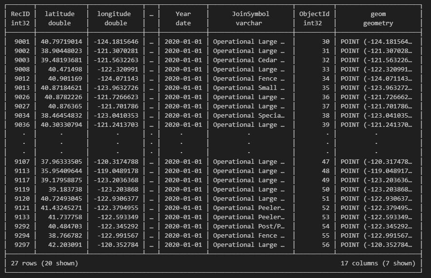
../_images/sawmill.png — Fig. 5.1 The entire sawmill dataset (columns and rows truncated).#

# View sawmill table schema
con.sql('''
    DESCRIBE sawmill
''')

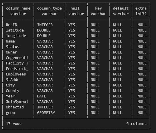
../_images/schema.png — Fig. 5.2 Sawmill table schema.#

Let’s run a query that sums sawmills by county (Fig. 5.3).

# Sum sawmills by county
con.sql('''
    SELECT County, COUNT(*) as Count
    FROM sawmill
    GROUP BY County
    ORDER BY count DESC
''')

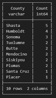
../_images/county.png — Fig. 5.3 Sum of total sawmills by county.#

Import the biomass database, then create and show the table.

# Import the Biomass dataset
con.sql("SELECT * FROM ST_Read('./biomass.shp')")

# Create biomass table from the shp file and show table
con.sql('''
    CREATE TABLE IF NOT EXISTS biomass as
    SELECT * FROM ST_Read('./biomass.shp')
''')
con.table('biomass')

View the biomass table schema, then sum the total megawatts of the plants by county, rounding the total to one decimal (Fig. 5.4).

# View biomass table schema
con.sql('''
    DESCRIBE biomass
''')

# Sum the total MW_Grid by county round to 1 decimal

con.sql('''
    SELECT County, ROUND(SUM(CAST(MW_Grid AS FLOAT)), 1) as Total_MW_Grid
    FROM biomass
    GROUP BY County
    ORDER BY Total_MW_Grid DESC
    LIMIT 15
''')

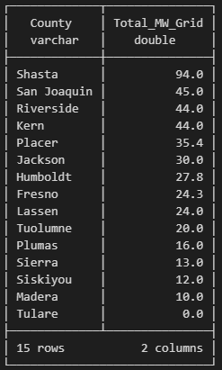
../_images/mw.png — Fig. 5.4 Sum of total megawats of biomass plants by county.#

5.5. Lewis’s Woodpecker#

Lewis’s Woodpecker (Melanerpes lewis) is a striking North American species of woodpecker named after 19th-century explorer Meriwether Lewis (Fig. 5.5). Although locally common, its breeding and migratory habits are not extensively known. Lewis’s Woodpeckers also engage in some un-woodpeckery behaviors such as hawking insects (Wikipedia). We’ll examine a dataset of Lewis’s species occurrence from eBird.

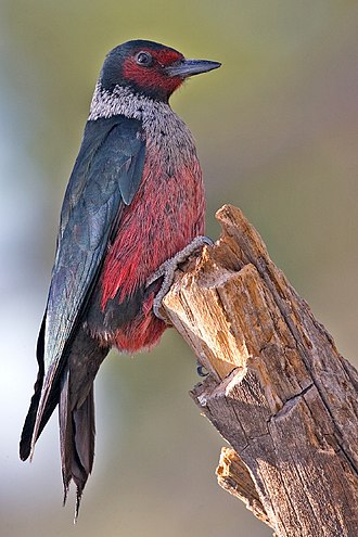
../_images/lewo.jpg — Fig. 5.5 Lewis’s Woodpecker (*Melanerpes lewis*). Photo courtesy of wikimedia.org.#

Installing the Geo Data Viewer plugin for VS Code will let you quickly view spatial datasets in a kepler.gl viewer. For example, if you clone the repo, right-click on the Lewis’s Woodpecker csv file in the test/lewo folder, and select View Map you’ll get a species distribution heatmap (Fig. 5.6).

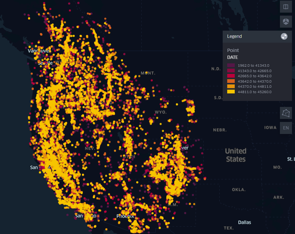
../_images/lewo_distrib.png — Fig. 5.6 Lewis’s Woodpecker distribution heatmap in the western United States.#

To analyze the woodpecker data, import the packages and connect to DuckDB.

# Import and connect
import duckdb
import leafmap
import pandas as pd
con = duckdb.connect()
con.install_extension("httpfs")
con.load_extension("httpfs")
con.install_extension("spatial")
con.load_extension("spatial")

The Lewis’s csv file is quite large, but DuckDB quickly runs through its ~140k rows. Create a table called lewo, short for Lewis’s Woodpecker. The csv file is in the repo’s test folder. Note using ST_Point to assign the latitude and longitude columns to geometry.

# Create lewo table and assign points lat lon points to geometry
sql = ("""
    CREATE TABLE lewo AS
    SELECT *,
        ST_Point(LONGITUDE, LATITUDE) as geometry
    FROM "./lewo/lewo.csv" 
""")
con.execute(sql)

# show the table
con.table("lewo")

If the FROM “./lew/lewo.csv” statement throws an error, try replacing the file path by right-clicking the file in your computer and selecting copy path, then passing that file path in place of “./lewo/low.csv”. For Windows, change the slashes to / instead of \ for the file path.

Then, count the total observations by state (Fig. 5.7).

# Count by state
con.sql('''
    SELECT STATE, COUNT(OBJECTID) as Count
    FROM lewo
    GROUP BY STATE
    ORDER BY Count DESC
    LIMIT 10
''')

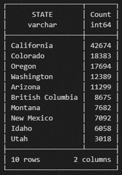
../_images/lewo_state.png — Fig. 5.7 Lewis’s Woodpecker counts by state.#

Select the Washington observations and name the new table ‘wash’.

# Select Washington state points and name the table wash
con.sql('''
    CREATE TABLE wash AS
    SELECT *
    FROM lewo
    WHERE STATE = 'Washington'
''')

Export the new table as a csv by converting it to a data frame and save in the test folder.

# Fetch the data from the wash table into a data frame
wash_df = con.execute("SELECT * FROM wash").fetchdf()

# Export the dataframe to a csv file in the test folder
wash_df.to_csv('test/wash.csv', index=False)

Right-clicking the csv file and selecting View Map produces a heat map. It shows that Lewis’s Woodpeckers prefer the Hood River and a certain elevation along the Pacific Crest (Fig. 5.8).

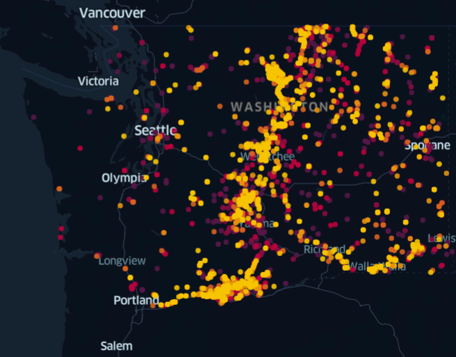
../_images/wash.png — Fig. 5.8 Distribution heatmap in Washington state of Lewis’s Woodpecker.#

Hopefully, these examples are enough to get you started. The resources below have more detailed examples and videos to go deeper. Make sure to practice and try out queries, joins, and other spatial functions with different datasets, including geosjson and geoparquet, to go beyond using shp and csv files.

5.6. Resources#

GEOG-414. The DuckDB portion of Qiusheng Wu’s Geography 414 course is a recommended way to expand your spatial SQL knowledge.
Spatial SQL. Matt Forrest’s text on using SQL in modern GIS is an excellent reference and starter for using SQL within a spatial context. Although the book could use a copyedit (many spelling errors) and better organization (figures disconnected from text, tutorials with more bullets/less text), everything is in the book that you will need to become a spatial SQL expert. The tutorials are relevant and guide you through critical beginner -> advanced workflows using spatial SQL.
SQL-QGIS Tip. You can use the ‘Execute SQL’ processing algorithm to run SQL queries on ANY vector layer within QGIS. Here’s an example of calculating group statistics on a vector layer. This also allows you to run SQL queries in a model.
Mark Litwintschik. This great data and geospatial blog features several tutorials running the DuckDB spatial extension.
Lonboard. Lonboard is a Python library for fast vector processing. The DuckDB Spatial tutorial links Lonboard to DuckDB and Python to create a heatmap.

SQL

Contents