2. GEE

Introduction to geospatial analysis in the cloud using Google Earth Engine

2.1. TL;DR

• Google Earth Engine is a rich resource with petabytes of datasets and the ability to analyze data in the cloud rapidly.

• GEE’s strength is cloud-based analysis, not visualization. For better visualization/cartographic tools, see Chapters 4, 6, and 8.

• See Chapter 4 and Geemap for a way to deploy Earth Engine using Python.

2.2. Scenario

You need to do a quick exploratory data analysis of above and below-ground carbon biomass for an area of interest near Lake Tahoe in the Central Sierra, California. A donor has asked you to do this by the end of the week. You go down the hall to the room where the map plotters are located and ask the ‘GIS guy’ for help. He peers up above his array of screens and says he’s busy working on a dozen other projects; he might be able to get you something in two weeks. He suggests you check out Google Earth Engine.

Yes! You’ve heard of this and think Google Earth will be easy. But when you check out Earth Engine and find a console with an empty map, the required Javascript coding is another universe, let alone language. Damn!

2.3. DIY

This scenario applies even if you don’t have a GIS guy down the hall with the defunct plotter! So, how do you DIY the donor’s needs?

Google Earth Engine may be one of the most ubiquitous free and open-source software packages for remote sensing and geospatial analysis. Technically, It isn’t free or open-source, but using it as an individual, nonprofit, or student is free. Its extensive library and ability to run computations in the cloud make it an exceptional resource for use anywhere you have an internet connection on any computer. And it’s not that difficult to start despite the use of Javascript!

The full code for this example can be found here.

Once you log into Earth Engine, search for ‘carbon’ in the search bar at the top of the page. Select Global Aboveground and Belowground Carbon Density Maps. In the lower left of the page, select See example (Fig. 2.1).

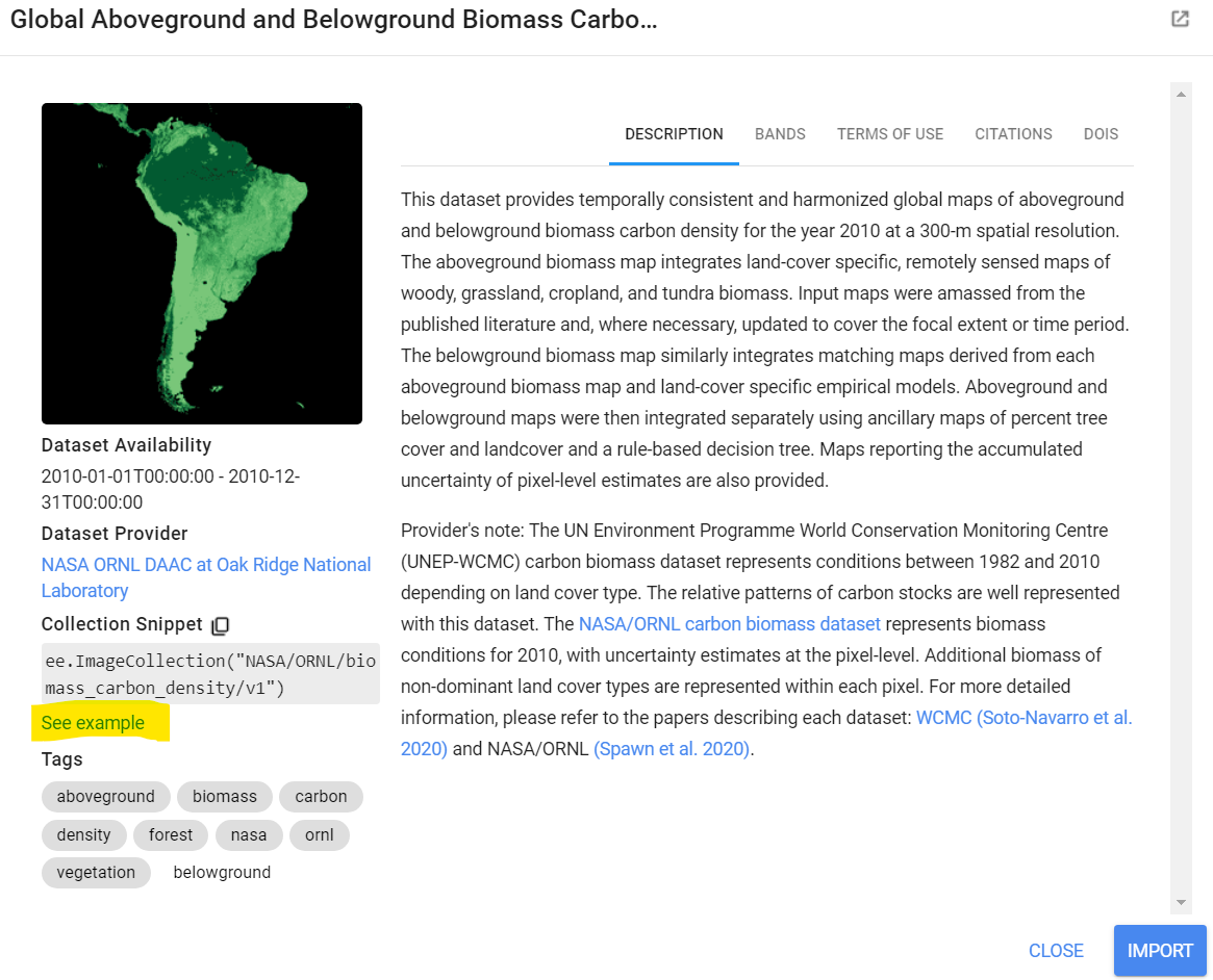
Fig. 2.1 Global above and belowground biomass carbon dataset.

That will open a new code editor with the following javascript code:

var dataset = ee.ImageCollection("NASA/ORNL/biomass_carbon_density/v1");

var visualization = {
  bands: ["agb"],
  min: -50.0,
  max: 80.0,
  palette: ["d9f0a3", "addd8e", "78c679", "41ab5d", "238443", "005a32"],
};

Map.setCenter(-60.0, 7.0, 4);

Map.addLayer(dataset, visualization, "Aboveground biomass carbon");

Clicking Run in the upper right of the interface will give you a basic map of aboveground biomass (Fig. 2.2).

Fig. 2.2 Aboveground biomass output.

You can zoom in or out and click the layer on or off. Selecting the Inspector in the upper right panel will allow you to click on any pixel in the map and get the information from the raster displayed (Fig. 2.3).

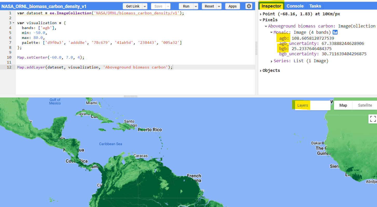
Fig. 2.3 Using the inspector tab in the console to get pixel information.

In this case, the Mosaic image has four bands related to above and belowground carbon, the latitude and longitude of a point clicked is (-68.16, 1.83), and the pixel size is 10 km. Add in the belowground (bgb) carbon with

var vis_b = {
  bands: ["bgb"],
  min: -50.0,
  max: 80.0,
  palette: ["D6BCB1", "AB8574", "784E3D", "3D2216", "26140C", "000000"],
};
Map.addLayer(dataset, vis_b, "Belowground biomass carbon");

You can zoom the map out and center to approximately world level by changing line 10 of the code:

Map.setCenter(-24.83, 19.88, 2);

Hit run or control + enter (windows) or command + enter (mac) to run the new code. Cleaning up the code and adding comments with // to explain what each section does is standard coding practice. The double forward slash allows you to add a comment that does not run when the code executes and is equivalent to the hashtag for Python. You can comment out any line of code by clicking on the line and typing the control/command enter on your keyboard. A reorganization will give you the following code and image (Fig. 2.4).

// Add global carbon density map
var dataset = ee.ImageCollection("NASA/ORNL/biomass_carbon_density/v1");

// Add visual parameter variables
var vis_a = {
  bands: ["agb"],
  min: -50.0,
  max: 80.0,
  palette: ["d9f0a3", "addd8e", "78c679", "41ab5d", "238443", "005a32"],
};

var vis_b = {
  bands: ["bgb"],
  min: -50.0,
  max: 80.0,
  palette: ["D6BCB1", "AB8574", "784E3D", "3D2216", "26140C", "000000"],
};

// Center map and add layers
Map.setCenter(-24.83, 19.88, 2);
Map.addLayer(dataset, vis_a, "Aboveground biomass carbon");
Map.addLayer(dataset, vis_b, "Belowground biomass carbon");

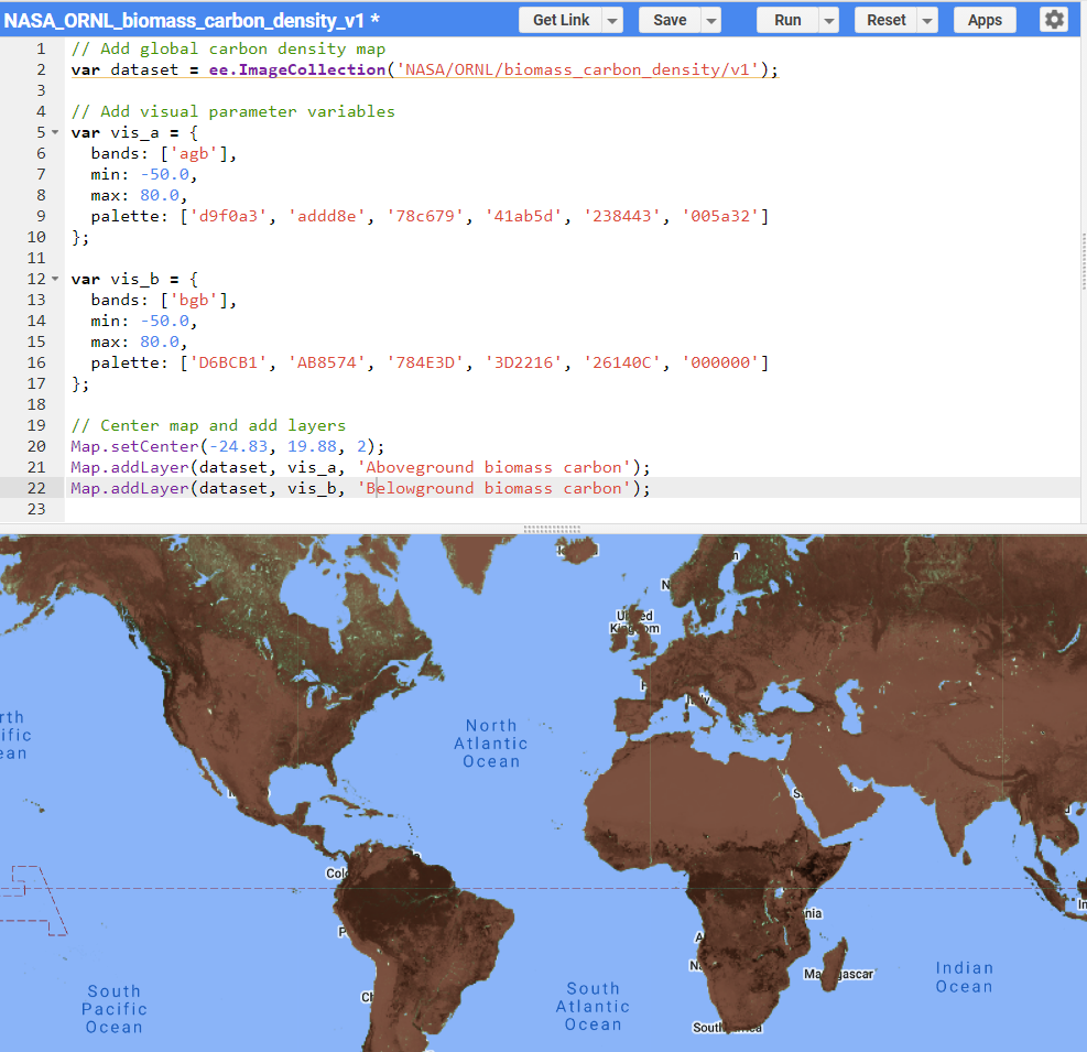
Fig. 2.4 Adding carbon density map at the world level.

Note that the belowground layer now shows up on top. Turn it off by clicking the checkmark in the layers tab, or to view it first, reverse the order of the code, e.g., line 22 moved to 21. You can alter the layer visibility by changing the Map.addLayer command with a true (visible) or false argument (added but visible) after the layer name:

Map.addLayer(dataset, vis_b, "Belowground biomass carbon", false);

Note the command structure: Map.addLayer(Dataset or feature to add to the map, visualization parameters, layer name, shown (true or false for shown/not shown), opacity). To see the arguments for any command, click Docs in the left panel and type the command name to search for it. Select the name and the API reference will appear.

2.4. AOI Clip

Getting back to the original request, you can clip the dataset to an area of interest, in this case, around Lake Tahoe. You can clip the map to datasets such as Tiger Lines for states or by country. Clipping by specific shape files requires you to upload the vector as a shape file into Earth Engine. This is fiddly and not as easy as dragging/dropping into Arc, QGIS, or online software such as Felt or Earth Blox. We’ll keep this to a simple box.

Turn off the map layers and zoom into your area of interest AOI, in this case near Lake Tahoe (Fig. 2.5).

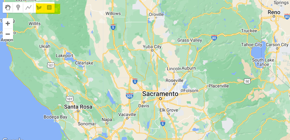
Fig. 2.5 Zooming to an area of interest. Note the highlighted rectangle/polygon buttons to add geometry vector layers.

Enter a search in the box at the top of Earth Engine, such as ‘South Lake Tahoe, CA, USA’. In the map pane, click on the square ‘Draw a Rectangle’ button highlighted and drag a square in the area (Fig. 2.6).

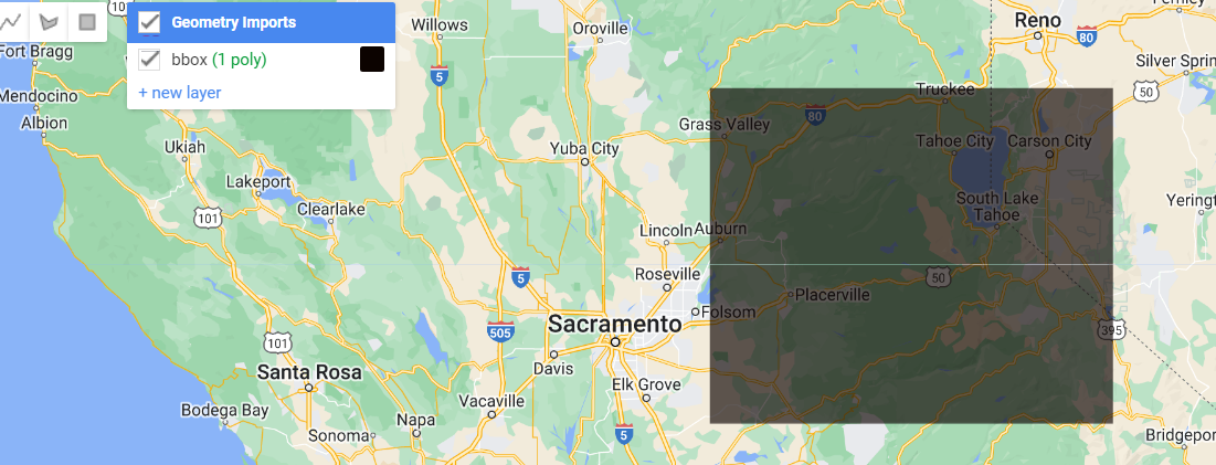
Fig. 2.6 Rectangle drawn to the area of interest. The default name will be geometry, here it is already re-named bbox.

This will add a layer in the imports section of the top of your code called geometry (var geometry: Polygon, 4 vertices). I have changed the name by double-clicking the layer name in the code editor to rename it ‘bbox’ (double-click geometry, type in bbox, and hit enter), but you can use the name geometry. If you use the default name or name it something else, remember to change the name from the code below from bbox to geometry (or your name). Under the dataset variable, change the code to the ImageCollection as follows:

// Add global carbon density map
var dataset = ee
  .ImageCollection("NASA/ORNL/biomass_carbon_density/v1")
  .map(function (image) {
    return image.clip(bbox);
  });

Note that the end of the dataset line no longer has a semicolon since the end of the code line now follows the bbox clip. Change the map center and zoom into your bounding box by changing the Map.setCenter function (line 21):

// Center map and add layers
Map.setCenter(-120.2348, 38.8744, 9);

Alternatively, change the line to Map.centerObject(bbox, 9) for a more memorable way to center. In the map pane, hover over Geometry Imports and unclick bbox. Run the code again (Fig. 2.7).

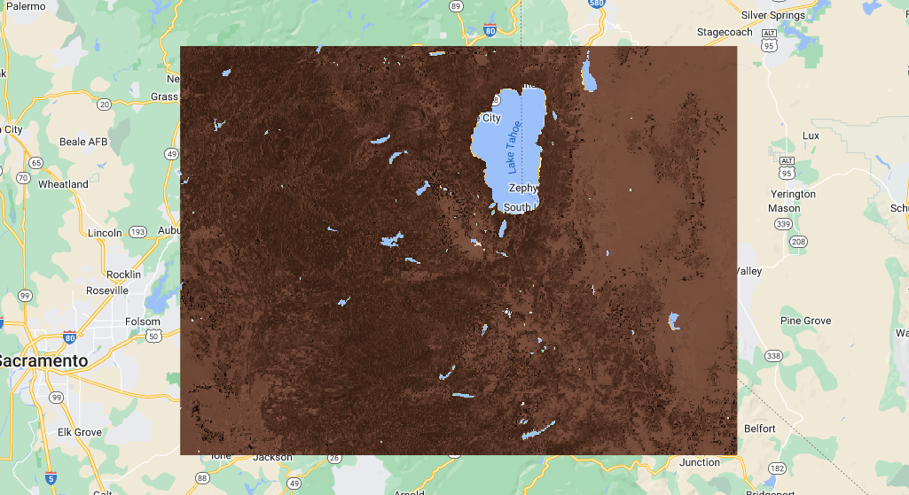
Fig. 2.7 Belowground biomass clipped to the area of interest.

Given the clash of colors for the brown and green carbon, it might help to change the basemap. This can be relatively simple or complicated in Earth Engine. Going to Snazzy Maps, selecting a basemap you like, and copying the javascript can make your work easier. In Snazzy, we’ll choose simple gray. Adding it to the map adds about 130 lines of code to your map, but there’s an easier way using the snazzy GitHub repository to reduce the total lines to two. Here, I used the Snazzy grayscale URL:

// Change basemap to snazzy subtle grayscale
var snazzy = require("users/aazuspan/snazzy:styles");
snazzy.addStyle("https://snazzymaps.com/style/15/subtle-grayscale", "Gray");

Once you hit enter, you will have ‘Gray’ as an additional map option in the middle right portion of your screen to go along with the default ‘Map’ and ‘Satellite’ options. Earth Engine has other defaults you can add without much code and can be found here. After adding the gray basemap the basemap selection bar changes (Fig. 2.8).

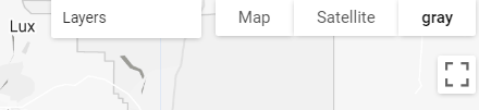
Fig. 2.8 Gray basemap bar after adding the grayscale map.

Altogether, the map now looks like Fig. 2.9 once the belowground layer is turned off.

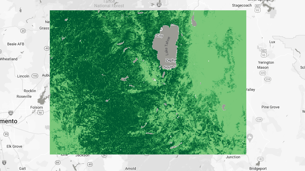
Fig. 2.9 Gray basemap bar after adding the grayscale map.

The full code is here. Congratulations, you’ve made your first Earth Engine map. Selecting the inspector pane in the top right allows you to click anywhere in the map to get coordinates and carbon values at the pixel level.

2.5. Geospatial EDA

This type of exploratory data analysis (EDA) is extraordinarily useful for looking at large datasets of multiple biotic and abiotic data types that the Earth Engine Catalog offers. You can search for any set in the catalog, click on the sample, and get an instantaneous data view. In reality, this is almost akin to no code. It also computes and adds any layer in the cloud, so it doesn’t matter how old or slow your computer is; you can run the geospatial computations in the cloud. This is a tremendous advantage, especially for more complex analyses.

For the map we just made, you would likely want to add functionality such as a legend showing carbon levels for each raster dataset and a graph with the range of carbon levels for the bounding box area.

2.6. Resources

There are many resources from getting started to the advanced use of Google Earth Engine:

• Spatial Thoughts, Ujaval Gandhi. End-to-End Google Earth Engine provides full course materials that start with setting up the Earth Engine environment and move into more advanced topics such as machine learning and change detection.

• Remote Sensing with GEE. If you want to get serious about Google Earth Engine, I highly recommend you read the free online Cloud-Based Remote Sensing with Google Earth Engine book by Rebecca Moore et al. This book is worth reading as a standalone remote sensing textbook and expertly guides you through everything from basic to complex geospatial analysis.

• Awesome-GEE. The Opengeos Awesome-GEE GitHub repo is a fantastic curated list of GEE resources. This incredible resource has everything from getting started to courses, papers, datasets, and more. You could lose yourself for days in here! — GEE Google Group. The Google Earth Engine Developers listserv is useful for answering many other questions, especially when you get stuck. — Awesome-GEE-Community-Catalog. Not to be confused with Awesome-GEE, the Awesome GEE Community Catalog is an equally awesome treasure trove of datasets ready for analysis and with sample code to start their use immediately.

• Visualization and Analysis of Brazil Floods 2024. This [tutorial] has an excellent workflow design and superb explanations of remote sensing theory and concepts in this tutorial. In addition, the tutorial contains very useful text and code for analyzing synthetic aperture radar (SAR) imagery.