8. R#
R is the definitive programming language for data analysis and visualization in academia. But it’s increasingly being used more broadly due to its ease of use and many analysis packages.
8.1. Similarities#
Javascript, Python, and R have similar code structures (Fig. 8.1).
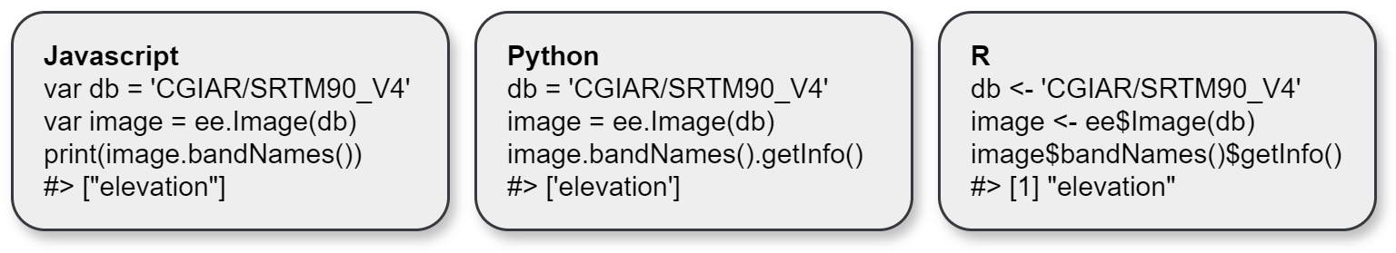
Fig. 8.1 Javascript, Python, and R code comparison. Adapted from rgee. Note that Python requires additional commands to run Earth Engine.#
It’s similar enough to organize each coding language in your head, almost like learning Spanish and Portuguese. It’s probably better to focus on one or the other. Still, you may find that one language sometimes offers better packages, processes data faster, or is preferred in a particular workplace.
Tip
R has the somewhat annoying symbol for variables or assignment operator of <-. Still, you can quickly create it using the keyboard shortcut Alt/Option and - (Alt and minus sign) in Windows/Mac.
8.2. Installation#
The RStudio desktop IDE is very good and only requires a two-step installation of R and RStudio. The IDE has a terminal, code section, installs packages through search, a variable/file panel, and a preview window showing maps, graphs, or other outputs.
If you don’t want to install yet another IDE, you can run R through VS Code with several basic to bespoke options:
Install R from CRAN.
Install the language server in R: ‘install.packages(“languageserver”)’
Go to extensions and install the R Extension Pack by Yuki Ueda. This will install R (the coding language) and R-LSP (provides language support and autocomplete for commands).
Install extra packages such as radian to make R easier to use. See the notes in the R extension in VS Code for additional recommendations, links, and installation instructions. This article is a concise guide for setup.
8.3. EDA#
The R library DataExplorer allows you to perform exploratory data analysis (EDA) on datasets. I’ve adapted this section from a post in datascienceplus.com from Raja 2018.
If you want to fast forward to creating an html report that opens in your browser, run the command create_report() after loading the package library and reading your dataset to a variable.
Tip
Package Installation. If you’re using RSTudio, you can also install packages by going to the packages tab in the Files, Plots, Packages pane (default location lower right), select Packages, Install, and enter the package name in the open window.
Running R Script. You can run each line of code entered by placing the cursor at the comment or line of code you want to run, then clicking the Run button in the upper right of the code pane (default location upper left), or using the control/command enter on your keyboard. You can also highlight an entire block or section of code and run it with the same command.
Install the Data Explorer package and load it.
install.packages('DataExplorer')
library(DataExplorer)
Download the chocoloate bar ratings dataset from kaggle and copy the path to wherever you store it.
Tip
If you use Windows OS, right-clicking on a file and selecting copying the path to the file will create a file pathway with backslashes rather than forward slashes and create an error when you run read.csv(). Install Path Copy Copy, right-click, select Show more options, and then Copy Unix Path.
Read the csv file, show the top 10 and total rows.
#read csv
cacao <- read.csv('./test/cacao.csv', header = T, stringsAsFactors = F)

#examine head and create summary statistics
head(cacao)
summary(cacao)
Running the head(cacao) line produces the top 6 rows and all columns in the console (Fig. 8.2).
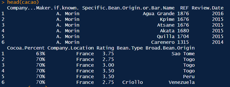
Fig. 8.2 Results from running head(cacao).#
It’s messy, but at least it confirms the dataset loaded. The summary command gives more information (Fig. 8.3).
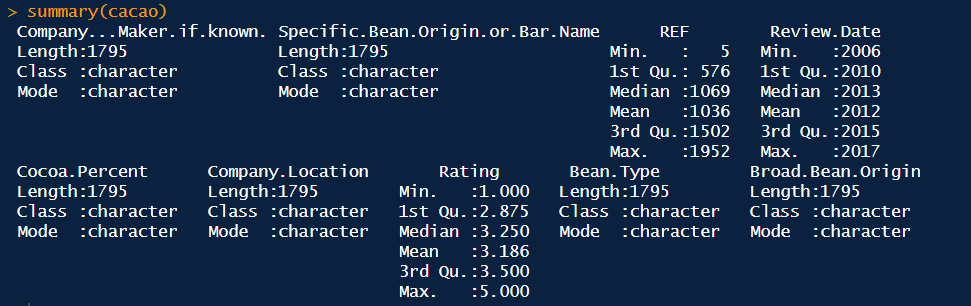
Fig. 8.3 Results from the summary(cacao) command.#
A better visual summary can be produced using plot_intro(cacao) (Fig. 8.4).
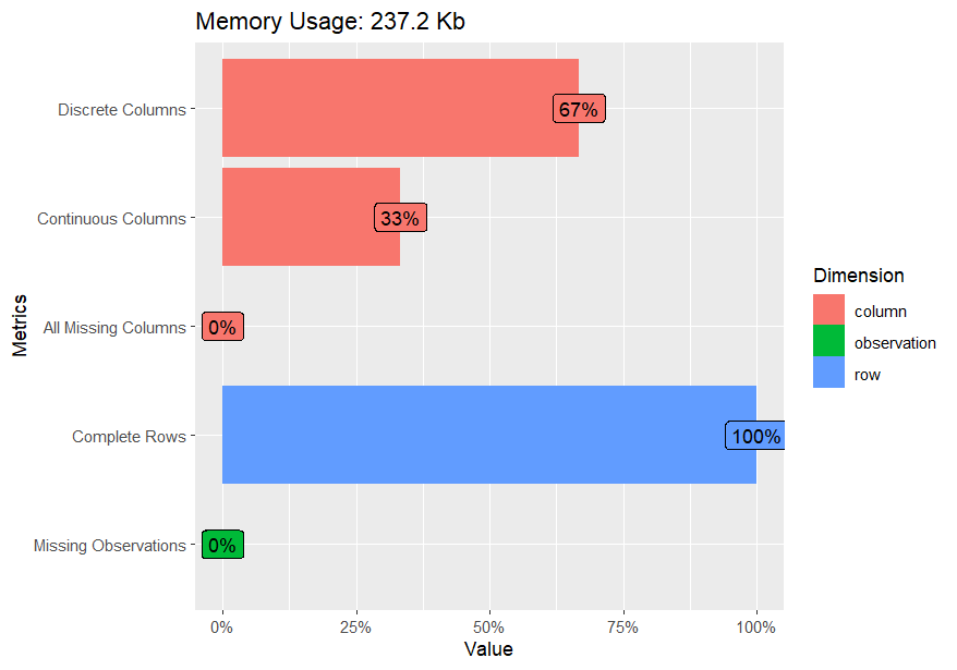
Fig. 8.4 Results from the plot_intro(cacao) command.#
Note the summary stats show the variable Cocoa.Percent is a character rather than a number due to the % sign attached to each value, and the review date needs to be changed to character. To fix this error, run the following:
# Fix Cocoa.Percent character error
cacao$Cocoa.Percent = as.numeric(gsub('%','',cacao$Cocoa.Percent))
cacao$Review.Date = as.character(cacao$Review.Date)
When you run head or summary again, the Cocoa.Percent column is now converted to numbers.
There are several functions to analyze and plot the dataset, such as categorical and continuous variables and other analyses. For example:
# variable dimension strings: variables, variable type, and total number
plot_str(cacao)
# missing values for each variable
plot_missing(cacao)
# variable histograms
plot_histogram(cacao)
# variable density plots
plot_density(cacao)
# variable bar plots
plot_bar(cacao)
# multivariate correlation analysis
plot_correlation(cacao, type = 'continuous','Review.Date')
For instance, the histogram plot shows distribution values for all the continuous variables. In this case, most cocoa percents are in the 70s, and ratings cluster around three (Fig. 8.5).
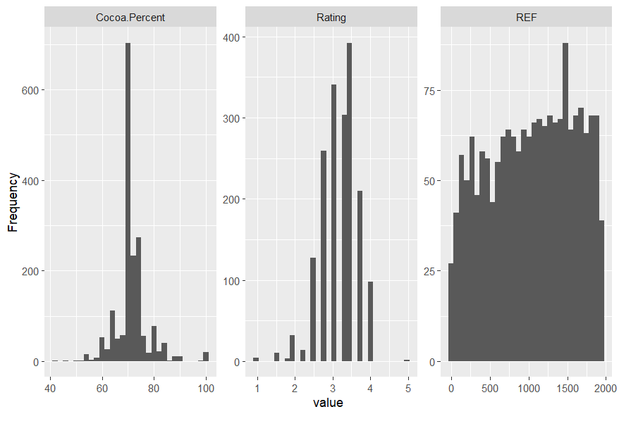
Fig. 8.5 Histogram plot.#
The simplified correlation analysis grouping Review.Dat shows a weak relationship between Rating and Cocoa.Percent (Fig. 8.6).
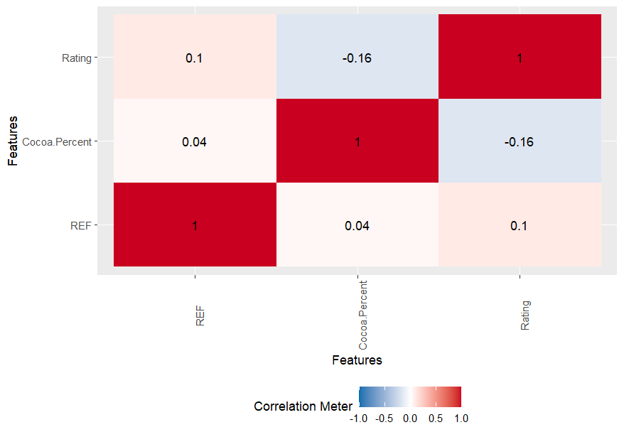
Fig. 8.6 Variable correlation plot.#
The create_report() function will run all of the EDA commands above, convert the outputs to an html file, and open the report in your default browser. This is useful if you want to enter one line and get a rapid summary of everything for the dataset. All of the above code runs very fast, even with large datasets. More details on the package can be found at the Introduction to DataExplorer site.
8.4. lidR#
Lidar (light detection and ranging) is frequently used for forest stand analysis. Let’s explore the lidR package to see its amazing 3D visualization and analysis capabilities. Not only does the package come with a book with excellent instructions to demo the package functions, but it also has a manageable las point cloud dataset [Roussel et al., 2023]. The following examples are excerpted from the book.
If you don’t want to use the provided dataset, the US Geological Service has a Lidar Explorer offering downloads of publicly available lidar datasets across the United States. Define an ROI on the map and download the tiled laz files. Beware, even a single tile can be huge. I downloaded a single tile in Mendocino County, CA, that was 1.3 GB in size and contained nearly 49 million points. By contrast, the las dataset from the lidR book is ‘only’ 2 mb and has a little less than 38,000 points.
## Install lidR import, read las file and plot
install.packages('lidR')
library(lidR)
LASfile <- system.file("extdata", "MixedConifer.laz", package="lidR")
las <- readLAS(LASfile, select = "xyzr", filter = "-drop_z_below 0")
plot(las, bg = "white", size = 4)
This will give you a popup window showing this dataset’s 3D point cloud of the lidar return, with the highest values in red and the lowest in blue (Fig. 8.7). Since the point cloud appears to be of a forest stand, you can discern tree outlines. If you left-click on the point cloud model, you can rotate the point cloud in 3 dimensions. Far out, man!
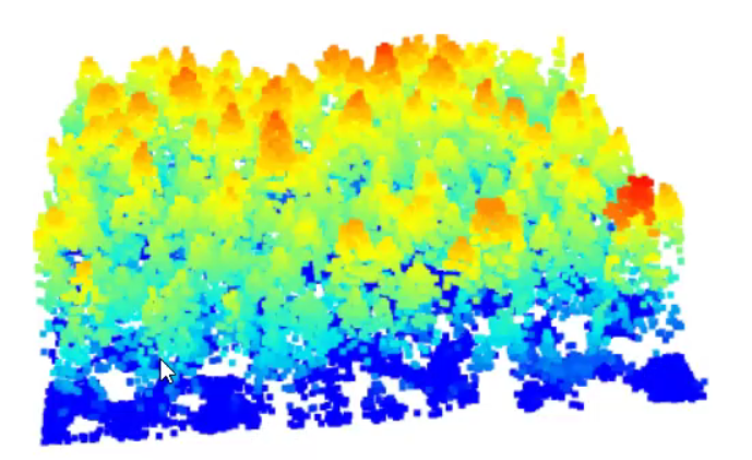
Fig. 8.7 Model of trees in 3d from las file.#
Rasterize a canopy height model and plot it. Note that the highest trees appear in the lower right corner, the same as in the 3D model (Fig. 8.8).
# Rasterize canopy height model
chm <- rasterize_canopy(las, 0.5, pitfree(subcircle = 0.2))
plot(chm, col = height.colors(50))
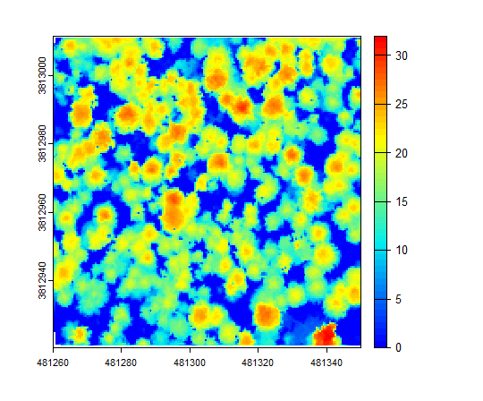
Fig. 8.8 Rasterized canopy height model.#
Locate the tree-top centers (Fig. 8.9).
# Locate the tree tops and plot
ttops <- locate_trees(las, lmf(ws = 5))
plot(sf::st_geometry(ttops), add = TRUE, pch = 3)
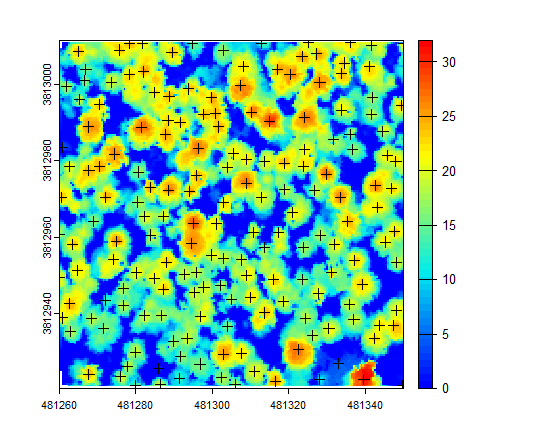
Fig. 8.9 Treetop centers in the rasterized canopy height model.#
You can also add the tree top centers to a 3d model (Fig. 8.10).
# Add 3d tree tops
add_treetops3d(x, ttops)
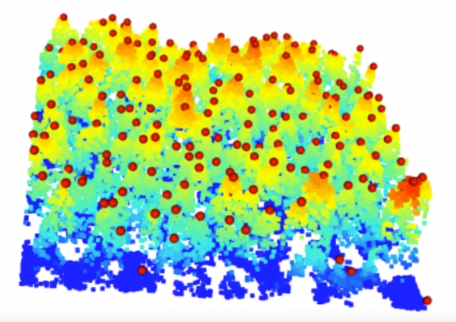
Fig. 8.10 Screenshot of the tree centers video in the 3d model.#
Finally, you can add custom metrics with a geometry argument that shows each tree as a convex hull shaded by height (Fig. 8.11).
metrics <- crown_metrics(las, func = ccm, geom = "convex")
plot(metrics["z_max"], pal = hcl.colors)
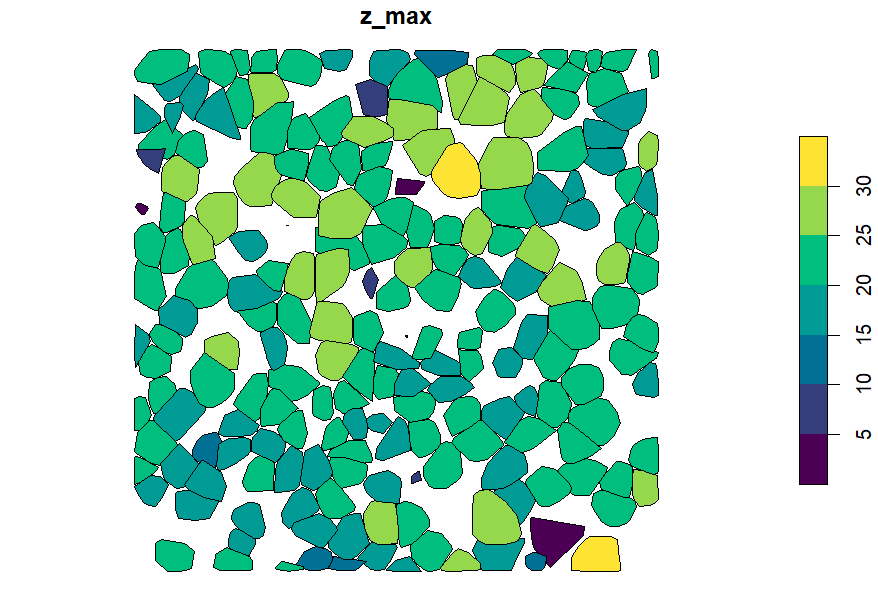
Fig. 8.11 Convex hulls of each tree in the canopy height model shaded by height.#
8.5. DuckDB#
Yes, you can execute DuckDB in R! DuckDB is everywhere, and because it uses SQL syntax, it looks similar to Python.
Install DuckDB, import the library, and create an in-memory database.
# Install and import duckdb
install.packages('duckdb')
library('duckdb')
con <- dbConnect(duckdb())
Create a simple table and insert two items into the table
# Create a table
dbExecute(con, "CREATE TABLE items(item VARCHAR, value DECIMAL(10, 2), count INTEGER)")
# Insert two items into the table
dbExecute(con, "INSERT INTO items VALUES ('jeans', 20.0, 1), ('hammer', 42.2, 2)")
Write a query for the table and show it in the R console.
# Query and print to console
res <- dbGetQuery(con, "SELECT * FROM items")
print(res)
Gives the output
    item value count
1  jeans  20.0     1
2 hammer  42.2     2
8.6. Resources#
These examples barely scratch the surface of what is available for geospatial R. The following resources provide a deeper dive:
Geocomputation with R. An excellent free and open source book hosted on Github and covers many aspects of geospatial analysis in R [Lovelace et al., 2019]. Spatial Data Science with Applications in R is another excellent resource [Pebesma and Bivand, 2023]. Both publications are great if you are new to R. Spatial Data Science is particularly good for explanations and figures accompanied by R codeblocks to show you how to assemble the code.
Neon intro to R. National Ecological Observatory Network from the US National Science Foundation introductory R tutorial.
The lidR package. LidR package book with tutorials.
Data Carpentry. Data carpentry R module. Data carpentry also has an intro to geospatial module.
Introduction to Statistical Learning. Look! You can do statistical learning in R or Python - Bonus!
r-spatial/rgee. An R library for Google Earth Engine. Chapter 6.4 of the Earth Engine Fundamentals and Applications is focused on the rgee package [Cardille et al., 2023].
lidR. Online book for the lidR package.
Data wrangling recipes in R. A nice resource for data preparation in R by Hilary Watt.