Abstract
A guide to understanding your data through exploratory data analysis (EDA) that includes systematic exploration, visualization, and statistical analysis. The chapter runs through an EDA workflow showing how to use various analysis packages, visualize data to show where problems may lie, and creates a report exportable as HTML.
EDA is the critical first step in any data analysis project. It involves:
Understanding structure - How is the data organized?
Identifying patterns - What trends or relationships exist?
Detecting anomalies - Are there outliers or errors?
Assessing data quality - Missing values, duplicates, inconsistencies?
Generating hypotheses - What insights might be worth investigating?
The process is iterative and visual, and will likely involve some data cleaning before data is ready for analaysis.
EDA Packages
Core tools for EDA include data analysis and profiling tools such as pandas, numpy, matplotlib, yadata-profiling, and missingno Table 1. R is also a great software platform for data analysis and EDA. The DataExplorer package quickly analyzes data and produces an HTML report. The closest Python equivalent is ydata-profiling that can also generate HTML reports.
Table 1:Python packages for EDA and R equivalents.
| Package | Purpose | R Equivalent |
|---|---|---|
| pandas | Data loading, manipulation, basic profiling | base R, dplyr |
| numpy | Numerical computations, statistics | base R |
| matplotlib, seaborn | Visualization | ggplot2, base graphics |
| ydata-profiling | Automated profiling reports | DataExplorer |
| missingno | Missing value visualization | vis_miss() |
Sample workflow
Let’s run through an example EDA workflow using a variety of packages and visualizations. We’ll first import dependencies then create a sample dataset.
# Import dependencies
import pandas as pd
import numpy as np
import matplotlib.pyplot as plt
import seaborn as sns
import missingno as msno

# Optional: Uncomment if you have ydata-profiling installed
# from ydata_profiling import ProfileReport

# Display settings
pd.set_option('display.max_columns', None)
pd.set_option('display.max_rows', 100)
pd.set_option('display.width', None)

# Visualization settings
plt.style.use('seaborn-v0_8-darkgrid')
sns.set_palette("husl")

print("✓ Libraries imported successfully!")
✓ Libraries imported successfully!
# Create a realistic environmental monitoring dataset
np.random.seed(42)
n_samples = 200

data = {
    'Site_ID': [f'SITE_{i:03d}' for i in range(1, n_samples + 1)],
    'Year': np.random.choice([2020, 2021, 2022, 2023], n_samples),
    'Latitude': np.random.uniform(35, 40, n_samples),
    'Longitude': np.random.uniform(-120, -115, n_samples),
    'Elevation_m': np.random.normal(2000, 500, n_samples),
    'Temperature_C': np.random.normal(15, 5, n_samples),
    'Precipitation_mm': np.random.exponential(50, n_samples),
    'Forest_Cover_%': np.random.normal(60, 20, n_samples),
    'Population_Density': np.random.exponential(100, n_samples),
    'Protected_Status': np.random.choice(['Protected', 'Unprotected', 'Buffer'], n_samples),
    'Land_Use': np.random.choice(['Forest', 'Agricultural', 'Urban', 'Shrubland'], n_samples)
}

df = pd.DataFrame(data)

# Introduce some missing values
df.loc[np.random.choice(df.index, 10), 'Temperature_C'] = np.nan
df.loc[np.random.choice(df.index, 8), 'Precipitation_mm'] = np.nan
df.loc[np.random.choice(df.index, 5), 'Forest_Cover_%'] = np.nan

# Add some duplicates
df = pd.concat([df, df.iloc[:5]], ignore_index=True)

print(f"Dataset created: {df.shape[0]} rows × {df.shape[1]} columns")
print(df.head())
Dataset created: 205 rows × 11 columns
Site_ID Year Latitude Longitude Elevation_m Temperature_C \
0 SITE_001 2022 35.157146 -119.741591 2170.877988 12.703196
1 SITE_002 2023 38.182052 -117.343227 2938.085420 10.750778
2 SITE_003 2020 36.571780 -117.296824 2475.211919 19.151679
3 SITE_004 2022 37.542853 -116.812850 1711.548172 10.719581
4 SITE_005 2022 39.537832 -116.369543 1550.792664 15.357831
Precipitation_mm Forest_Cover_% Population_Density Protected_Status \
0 58.927692 48.896009 204.603346 Unprotected
1 94.588599 97.623141 152.503006 Unprotected
2 14.361976 31.039722 83.705511 Unprotected
3 33.610883 16.023881 134.112679 Protected
4 12.500656 68.800289 210.796910 Buffer
Land_Use
0 Urban
1 Agricultural
2 Shrubland
3 Urban
4 Shrubland
Printing df.head gives you an initial glimpse of the data and fields in a tabular format. We’ll look at data structure next.
# Basic shape and structure
print("=" * 60)
print("DATASET STRUCTURE")
print("=" * 60)
print(f"Shape: {df.shape} ({df.shape[0]} rows, {df.shape[1]} columns)")
print(f"\nColumn Names and Types:")
print(df.dtypes)

# More detailed info
print("\n" + "=" * 60)
print("DETAILED INFO")
print("=" * 60)
df.info()

# First and last rows
print("\n" + "=" * 60)
print("FIRST FEW ROWS")
print("=" * 60)
print(df.head())

print("\nLAST FEW ROWS")
print(df.tail())
============================================================
DATASET STRUCTURE
============================================================
Shape: (205, 11) (205 rows, 11 columns)
Column Names and Types:
Site_ID object
Year int64
Latitude float64
Longitude float64
Elevation_m float64
Temperature_C float64
Precipitation_mm float64
Forest_Cover_% float64
Population_Density float64
Protected_Status object
Land_Use object
dtype: object
============================================================
DETAILED INFO
============================================================
<class 'pandas.core.frame.DataFrame'>
RangeIndex: 205 entries, 0 to 204
Data columns (total 11 columns):
# Column Non-Null Count Dtype
--- ------ -------------- -----
0 Site_ID 205 non-null object
1 Year 205 non-null int64
2 Latitude 205 non-null float64
3 Longitude 205 non-null float64
4 Elevation_m 205 non-null float64
5 Temperature_C 196 non-null float64
6 Precipitation_mm 197 non-null float64
7 Forest_Cover_% 200 non-null float64
8 Population_Density 205 non-null float64
9 Protected_Status 205 non-null object
10 Land_Use 205 non-null object
dtypes: float64(7), int64(1), object(3)
memory usage: 17.7+ KB
============================================================
FIRST FEW ROWS
============================================================
Site_ID Year Latitude Longitude Elevation_m Temperature_C \
0 SITE_001 2022 35.157146 -119.741591 2170.877988 12.703196
1 SITE_002 2023 38.182052 -117.343227 2938.085420 10.750778
2 SITE_003 2020 36.571780 -117.296824 2475.211919 19.151679
3 SITE_004 2022 37.542853 -116.812850 1711.548172 10.719581
4 SITE_005 2022 39.537832 -116.369543 1550.792664 15.357831
Precipitation_mm Forest_Cover_% Population_Density Protected_Status \
0 58.927692 48.896009 204.603346 Unprotected
1 94.588599 97.623141 152.503006 Unprotected
2 14.361976 31.039722 83.705511 Unprotected
3 33.610883 16.023881 134.112679 Protected
4 12.500656 68.800289 210.796910 Buffer
Land_Use
0 Urban
1 Agricultural
2 Shrubland
3 Urban
4 Shrubland
LAST FEW ROWS
Site_ID Year Latitude Longitude Elevation_m Temperature_C \
200 SITE_001 2022 35.157146 -119.741591 2170.877988 12.703196
201 SITE_002 2023 38.182052 -117.343227 2938.085420 10.750778
202 SITE_003 2020 36.571780 -117.296824 2475.211919 19.151679
203 SITE_004 2022 37.542853 -116.812850 1711.548172 10.719581
204 SITE_005 2022 39.537832 -116.369543 1550.792664 15.357831
Precipitation_mm Forest_Cover_% Population_Density Protected_Status \
200 58.927692 48.896009 204.603346 Unprotected
201 94.588599 97.623141 152.503006 Unprotected
202 14.361976 31.039722 83.705511 Unprotected
203 33.610883 16.023881 134.112679 Protected
204 12.500656 68.800289 210.796910 Buffer
Land_Use
200 Urban
201 Agricultural
202 Shrubland
203 Urban
204 Shrubland
This is so exciting! The first dataset structure table is critical to understand the types of data in your dataset. One of the most common problems in datasets are fields assigned text values when they should be integers or vice versa.
Missing data can bias results or reduce sample size. Always investigate!
Summary Statistics
# Missing value analysis
print("=" * 60)
print("MISSING VALUES")
print("=" * 60)

# Count and percentage
missing = pd.DataFrame({
    'Count': df.isnull().sum(),
    'Percentage': (df.isnull().sum() / len(df) * 100).round(2)
})
missing = missing[missing['Count'] > 0].sort_values('Count', ascending=False)

if len(missing) > 0:
    print(missing)
else:
    print("No missing values found (but we introduced some, so they should appear)")

# Total missing
total_cells = df.shape[0] * df.shape[1]
total_missing = df.isnull().sum().sum()
print(f"\nTotal missing cells: {total_missing} / {total_cells} ({total_missing/total_cells*100:.2f}%)")

# Duplicates
print("\n" + "=" * 60)
print("DUPLICATES")
print("=" * 60)
duplicates = df.duplicated().sum()
print(f"Duplicate rows: {duplicates}")

if duplicates > 0:
    print(f"\nDuplicate rows:")
    print(df[df.duplicated(keep=False)].sort_values(by=list(df.columns)))
============================================================
MISSING VALUES
============================================================
Count Percentage
Temperature_C 9 4.39
Precipitation_mm 8 3.90
Forest_Cover_% 5 2.44
Total missing cells: 22 / 2255 (0.98%)
============================================================
DUPLICATES
============================================================
Duplicate rows: 5
Duplicate rows:
Site_ID Year Latitude Longitude Elevation_m Temperature_C \
0 SITE_001 2022 35.157146 -119.741591 2170.877988 12.703196
200 SITE_001 2022 35.157146 -119.741591 2170.877988 12.703196
1 SITE_002 2023 38.182052 -117.343227 2938.085420 10.750778
201 SITE_002 2023 38.182052 -117.343227 2938.085420 10.750778
2 SITE_003 2020 36.571780 -117.296824 2475.211919 19.151679
202 SITE_003 2020 36.571780 -117.296824 2475.211919 19.151679
3 SITE_004 2022 37.542853 -116.812850 1711.548172 10.719581
203 SITE_004 2022 37.542853 -116.812850 1711.548172 10.719581
4 SITE_005 2022 39.537832 -116.369543 1550.792664 15.357831
204 SITE_005 2022 39.537832 -116.369543 1550.792664 15.357831
Precipitation_mm Forest_Cover_% Population_Density Protected_Status \
0 58.927692 48.896009 204.603346 Unprotected
200 58.927692 48.896009 204.603346 Unprotected
1 94.588599 97.623141 152.503006 Unprotected
201 94.588599 97.623141 152.503006 Unprotected
2 14.361976 31.039722 83.705511 Unprotected
202 14.361976 31.039722 83.705511 Unprotected
3 33.610883 16.023881 134.112679 Protected
203 33.610883 16.023881 134.112679 Protected
4 12.500656 68.800289 210.796910 Buffer
204 12.500656 68.800289 210.796910 Buffer
Land_Use
0 Urban
200 Urban
1 Agricultural
201 Agricultural
2 Shrubland
202 Shrubland
3 Urban
203 Urban
4 Shrubland
204 Shrubland
Missingno
# Visualize missing values
fig, axes = plt.subplots(2, 2, figsize=(14, 8))

# Matrix visualization - shows missing pattern
plt.subplot(2, 2, 1)
msno.matrix(df, ax=plt.gca(), sparkline=False)
plt.title('Missing Value Matrix', fontweight='bold')

# Bar chart - shows count by column
plt.subplot(2, 2, 2)
msno.bar(df, ax=plt.gca())
plt.title('Missing Value Counts', fontweight='bold')

# Heatmap - shows correlation of missingness
plt.subplot(2, 2, 3)
msno.heatmap(df, ax=plt.gca())
plt.title('Missing Value Correlation', fontweight='bold')

plt.tight_layout()
plt.show()

print("Interpretation:")
print("- Matrix: White lines show missing data locations")
print("- Bar: Heights show how many values are present in each column")
print("- Heatmap: Shows which missing values tend to occur together")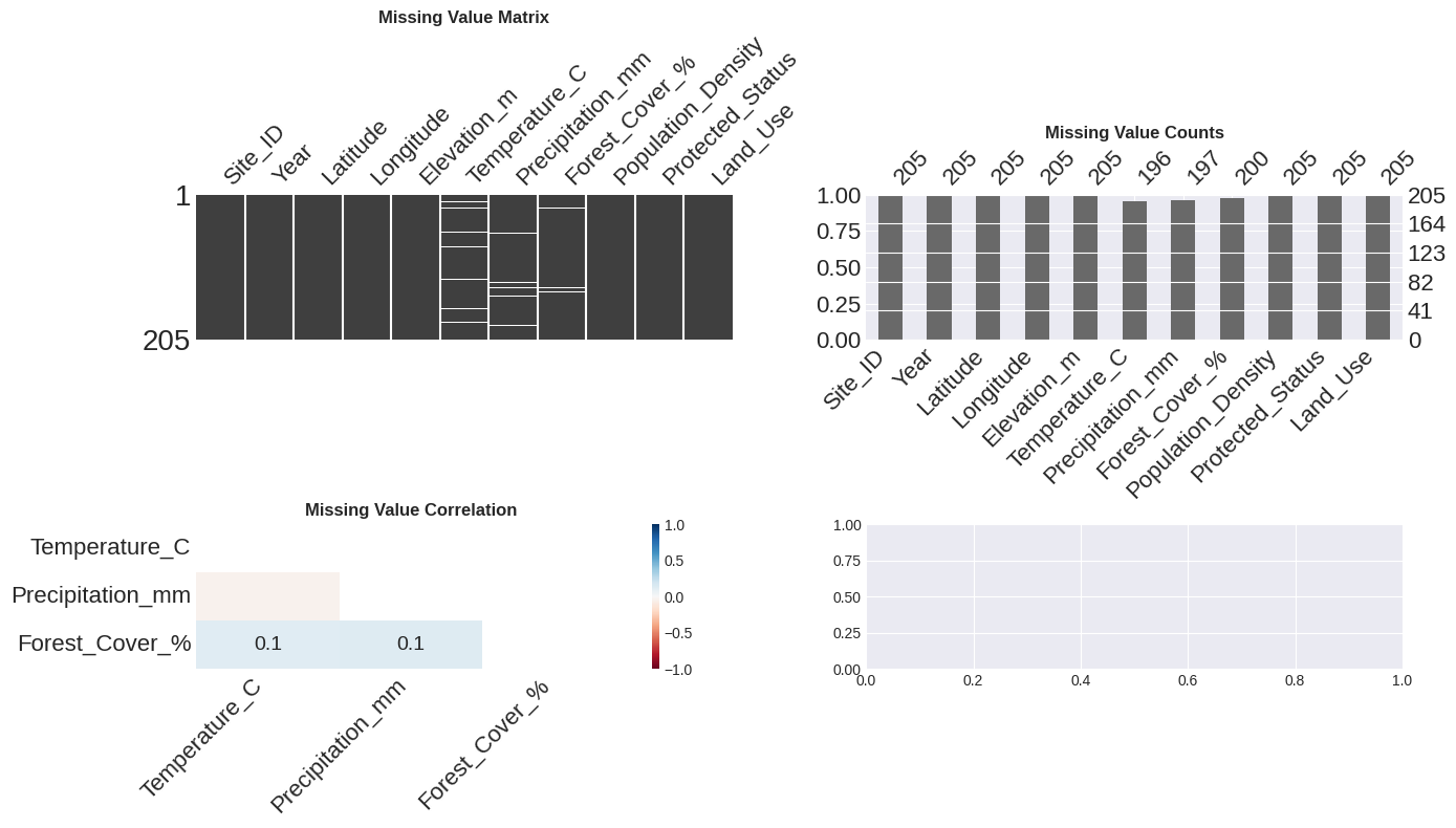
Interpretation:
- Matrix: White lines show missing data locations
- Bar: Heights show how many values are present in each column
- Heatmap: Shows which missing values tend to occur together
Descriptive statistics.
# Statistical summary of numerical columns
print("=" * 60)
print("DESCRIPTIVE STATISTICS")
print("=" * 60)
print(df.describe().round(2))

# Get specific statistics
print("\n" + "=" * 60)
print("SKEWNESS AND KURTOSIS")
print("=" * 60)
numeric_cols = df.select_dtypes(include=[np.number]).columns
for col in numeric_cols:
    skew = df[col].skew()
    kurt = df[col].kurtosis()
    print(f"{col:25} - Skewness: {skew:7.2f}  |  Kurtosis: {kurt:7.2f}")

# Categorical summary
print("\n" + "=" * 60)
print("CATEGORICAL VARIABLES")
print("=" * 60)
categorical_cols = df.select_dtypes(include=['object']).columns
for col in categorical_cols:
    print(f"\n{col}:")
    print(df[col].value_counts())
    print(f"Unique values: {df[col].nunique()}")
============================================================
DESCRIPTIVE STATISTICS
============================================================
Year Latitude Longitude Elevation_m Temperature_C \
count 205.00 205.00 205.00 205.00 196.00
mean 2021.59 37.54 -117.48 1976.70 15.08
std 1.12 1.46 1.52 515.26 5.00
min 2020.00 35.03 -119.95 764.18 1.52
25% 2021.00 36.25 -118.75 1603.56 11.77
50% 2022.00 37.59 -117.36 1972.23 15.08
75% 2023.00 38.81 -116.23 2316.39 18.49
max 2023.00 39.95 -115.04 3539.44 28.16
Precipitation_mm Forest_Cover_% Population_Density
count 197.00 200.00 205.00
mean 57.31 61.68 99.03
std 55.06 19.81 95.00
min 0.32 2.07 0.58
25% 14.36 48.97 32.04
50% 44.87 62.48 76.13
75% 84.60 74.27 133.51
max 309.11 108.07 513.95
============================================================
SKEWNESS AND KURTOSIS
============================================================
Year - Skewness: -0.13 | Kurtosis: -1.33
Latitude - Skewness: -0.05 | Kurtosis: -1.25
Longitude - Skewness: -0.08 | Kurtosis: -1.22
Elevation_m - Skewness: 0.13 | Kurtosis: -0.27
Temperature_C - Skewness: 0.07 | Kurtosis: -0.00
Precipitation_mm - Skewness: 1.58 | Kurtosis: 3.09
Forest_Cover_% - Skewness: -0.22 | Kurtosis: -0.05
Population_Density - Skewness: 1.96 | Kurtosis: 4.87
============================================================
CATEGORICAL VARIABLES
============================================================
Site_ID:
Site_ID
SITE_005 2
SITE_004 2
SITE_003 2
SITE_002 2
SITE_001 2
..
SITE_071 1
SITE_072 1
SITE_073 1
SITE_074 1
SITE_062 1
Name: count, Length: 200, dtype: int64
Unique values: 200
Protected_Status:
Protected_Status
Protected 78
Unprotected 69
Buffer 58
Name: count, dtype: int64
Unique values: 3
Land_Use:
Land_Use
Shrubland 58
Agricultural 52
Urban 51
Forest 44
Name: count, dtype: int64
Unique values: 4
Distribution analysis
and visualizing distributions
# Create histograms and box plots for numeric columns
numeric_cols = df.select_dtypes(include=[np.number]).columns

fig, axes = plt.subplots(4, 2, figsize=(14, 12))
axes = axes.flatten()

for idx, col in enumerate(numeric_cols[:8]):
    # Histogram with KDE
    axes[idx].hist(df[col].dropna(), bins=20, edgecolor='black', alpha=0.7, color='steelblue')
    axes[idx].set_title(f'{col}\n(n={df[col].notna().sum()}, missing={df[col].isna().sum()})',
                        fontweight='bold', fontsize=10)
    axes[idx].set_ylabel('Frequency')
    axes[idx].grid(True, alpha=0.3)

plt.tight_layout()
plt.show()

# Box plots for outlier detection
fig, axes = plt.subplots(2, 3, figsize=(14, 8))
axes = axes.flatten()

for idx, col in enumerate(numeric_cols[:6]):
    sns.boxplot(y=df[col], ax=axes[idx], color='lightblue')
    axes[idx].set_title(f'{col}', fontweight='bold')
    axes[idx].grid(True, alpha=0.3, axis='y')

plt.tight_layout()
plt.show()

print("Interpretation:")
print("- Histograms show the distribution shape")
print("- Box plots show median, quartiles, and potential outliers")
print("- Points beyond whiskers may be outliers worth investigating")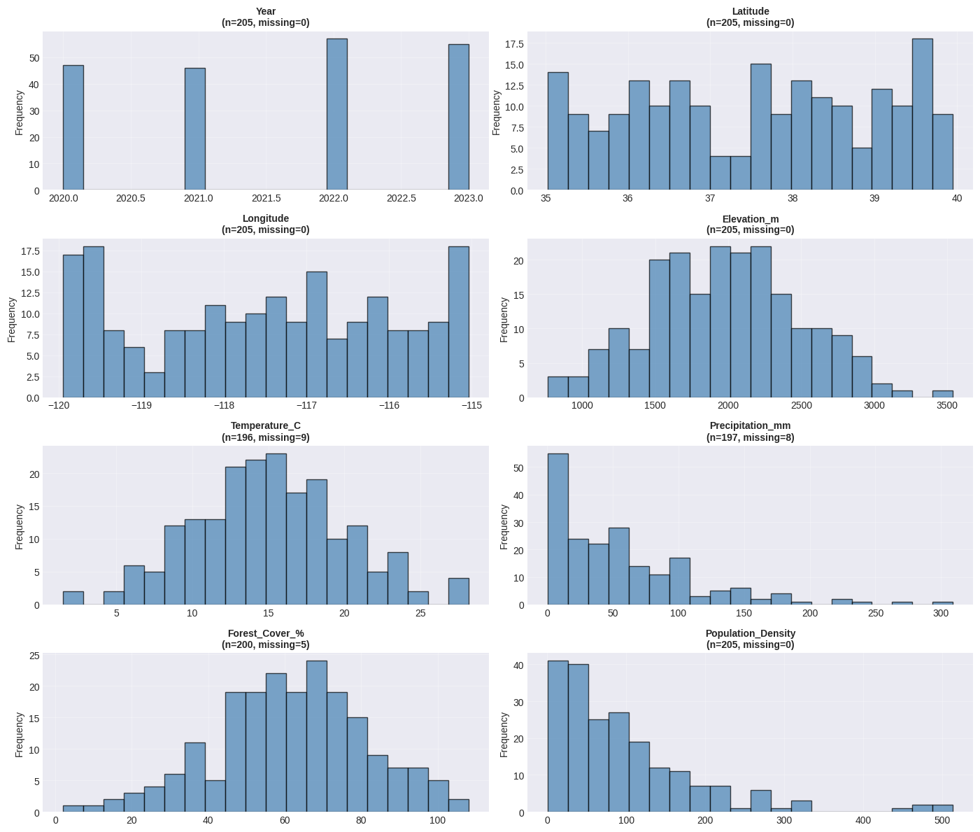
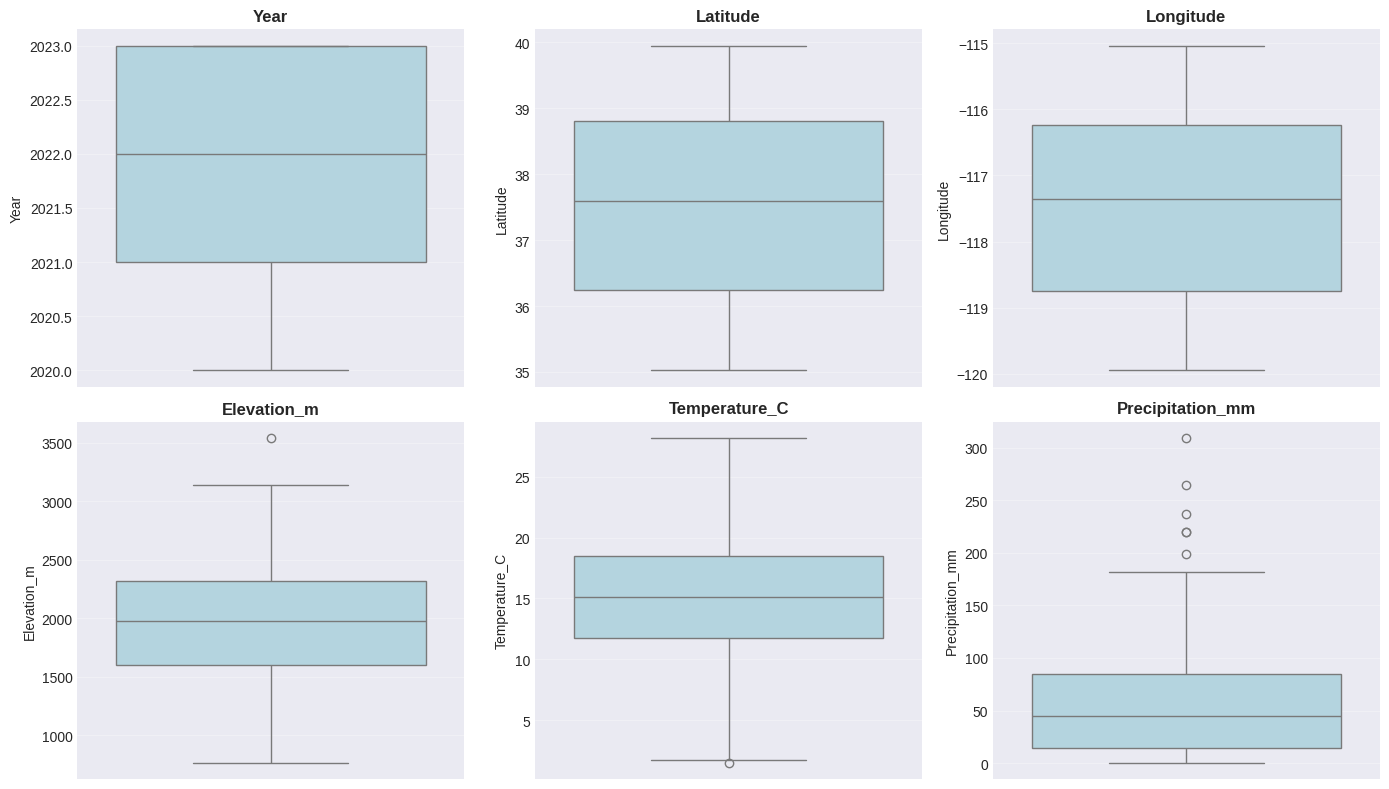
Interpretation:
- Histograms show the distribution shape
- Box plots show median, quartiles, and potential outliers
- Points beyond whiskers may be outliers worth investigating
Correlation matrix
# Calculate correlation matrix
corr_matrix = df.corr(numeric_only=True)

# Heatmap visualization
fig, ax = plt.subplots(figsize=(10, 8))
sns.heatmap(corr_matrix, annot=True, fmt='.2f', cmap='coolwarm', center=0,
            square=True, linewidths=1, cbar_kws={"shrink": 0.8}, ax=ax)
ax.set_title('Correlation Matrix: Numerical Variables', fontsize=13, fontweight='bold', pad=15)
plt.tight_layout()
plt.show()

# Find strongest correlations (excluding diagonal)
print("=" * 60)
print("STRONGEST CORRELATIONS")
print("=" * 60)

# Get correlations above threshold (excluding 1.0)
corr_list = []
for i in range(len(corr_matrix.columns)):
    for j in range(i+1, len(corr_matrix.columns)):
        corr_list.append({
            'Variable1': corr_matrix.columns[i],
            'Variable2': corr_matrix.columns[j],
            'Correlation': corr_matrix.iloc[i, j]
        })

corr_df = pd.DataFrame(corr_list).sort_values('Correlation', key=abs, ascending=False)
print(corr_df.head(10).to_string(index=False))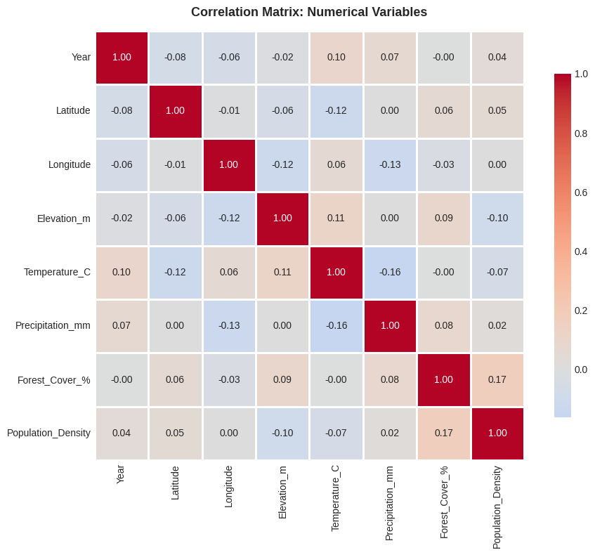
============================================================
STRONGEST CORRELATIONS
============================================================
       Variable1          Variable2  Correlation
  Forest_Cover_% Population_Density     0.166868
   Temperature_C   Precipitation_mm    -0.163705
       Longitude   Precipitation_mm    -0.125927
        Latitude      Temperature_C    -0.119565
       Longitude        Elevation_m    -0.115227
     Elevation_m      Temperature_C     0.114732
            Year      Temperature_C     0.102317
     Elevation_m Population_Density    -0.095198
     Elevation_m     Forest_Cover_%     0.086845
Precipitation_mm     Forest_Cover_%     0.084183
ydata-profiling
The ydata-profiling package is the Python equivalent of R’s DataExplorer. It generates comprehensive HTML reports with one line of code.
# Example: Automated profiling with ydata-profiling
# Uncomment below to run (requires: pip install ydata-profiling)

"""
from ydata_profiling import ProfileReport

# Generate profile report
profile = ProfileReport(df, title="Environmental Data Profile", minimal=False)

# Save to HTML file
profile.to_file("eda_report.html")

# Or display in Jupyter
# profile.to_notebook_iframe()
"""

# Manual equivalent when ydata-profiling is not available
print("=" * 60)
print("EDA SUMMARY (Manual Alternative to ydata-profiling)")
print("=" * 60)

summary = {
    'Total Rows': len(df),
    'Total Columns': len(df.columns),
    'Numeric Columns': len(df.select_dtypes(include=[np.number]).columns),
    'Categorical Columns': len(df.select_dtypes(include=['object']).columns),
    'Total Missing': df.isnull().sum().sum(),
    'Duplicate Rows': df.duplicated().sum(),
    'Memory Usage (MB)': df.memory_usage(deep=True).sum() / 1024**2
}

for key, value in summary.items():
    if isinstance(value, float):
        print(f"{key:.<35} {value:.2f}")
    else:
        print(f"{key:.<35} {value}")
============================================================
EDA SUMMARY (Manual Alternative to ydata-profiling)
============================================================
Total Rows......................... 205
Total Columns...................... 11
Numeric Columns.................... 8
Categorical Columns................ 3
Total Missing...................... 22
Duplicate Rows..................... 5
Memory Usage (MB).................. 0.05
Categorical Data Analysis
# Categorical data visualization
categorical_cols = df.select_dtypes(include=['object']).columns

fig, axes = plt.subplots(1, len(categorical_cols), figsize=(14, 4))
if len(categorical_cols) == 1:
    axes = [axes]

for idx, col in enumerate(categorical_cols):
    value_counts = df[col].value_counts()
    axes[idx].barh(value_counts.index, value_counts.values, color='steelblue', edgecolor='black')
    axes[idx].set_title(f'{col}\n(n={len(value_counts)} categories)', fontweight='bold')
    axes[idx].set_xlabel('Count')
    axes[idx].grid(True, alpha=0.3, axis='x')

plt.tight_layout()
plt.show()

# Cross-tabulation analysis
print("=" * 60)
print("CROSSTAB: Protected_Status × Land_Use")
print("=" * 60)
if 'Protected_Status' in df.columns and 'Land_Use' in df.columns:
    crosstab = pd.crosstab(df['Protected_Status'], df['Land_Use'], margins=True)
    print(crosstab)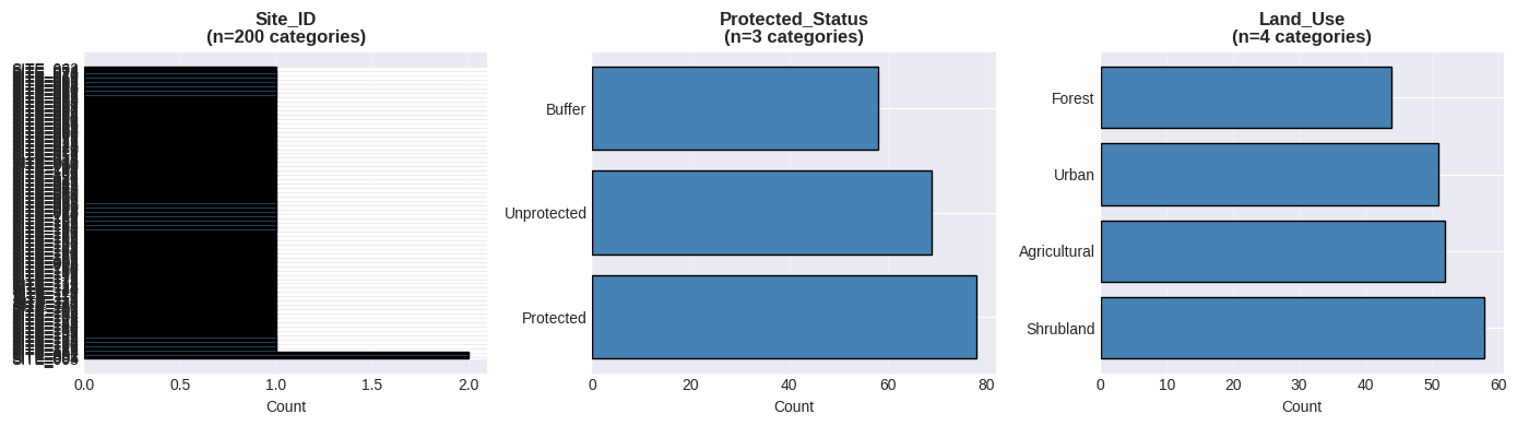
============================================================
CROSSTAB: Protected_Status × Land_Use
============================================================
Land_Use          Agricultural  Forest  Shrubland  Urban  All
Protected_Status
Buffer                      17      10         18     13   58
Protected                   18      21         19     20   78
Unprotected                 17      13         21     18   69
All                         52      44         58     51  205
EDA function
def quick_eda(df, name="Dataset"):
    """
    Perform quick EDA on a DataFrame

    Parameters:
    -----------
    df : pandas.DataFrame
        The dataset to analyze
    name : str
        Name of the dataset for reporting
    """
    print(f"\n{'='*70}")
    print(f"EXPLORATORY DATA ANALYSIS: {name}")
    print(f"{'='*70}\n")

    # Shape and types
    print(f"Shape: {df.shape[0]} rows × {df.shape[1]} columns")
    print(f"Memory: {df.memory_usage(deep=True).sum() / 1024**2:.2f} MB\n")

    # Missing values
    missing_pct = (df.isnull().sum() / len(df) * 100)
    if missing_pct.sum() > 0:
        print("Missing Values:")
        print(missing_pct[missing_pct > 0].sort_values(ascending=False))
        print()

    # Duplicates
    print(f"Duplicates: {df.duplicated().sum()}")

    # Data types
    print("\nData Types:")
    print(df.dtypes.value_counts())

    # Numerical summary
    print("\n" + "-"*70)
    print("NUMERICAL VARIABLES")
    print("-"*70)
    print(df.describe().round(2))

    # Categorical summary
    cat_cols = df.select_dtypes(include=['object']).columns
    if len(cat_cols) > 0:
        print("\n" + "-"*70)
        print("CATEGORICAL VARIABLES")
        print("-"*70)
        for col in cat_cols:
            print(f"\n{col}: {df[col].nunique()} unique values")
            print(df[col].value_counts().head(3))

    print(f"\n{'='*70}\n")

# Test the function
quick_eda(df, name="Environmental Monitoring Data")
======================================================================
EXPLORATORY DATA ANALYSIS: Environmental Monitoring Data
======================================================================

Shape: 205 rows × 11 columns
Memory: 0.05 MB

Missing Values:
Temperature_C       4.390244
Precipitation_mm    3.902439
Forest_Cover_%      2.439024
dtype: float64

Duplicates: 5

Data Types:
float64    7
object     3
int64      1
Name: count, dtype: int64

----------------------------------------------------------------------
NUMERICAL VARIABLES
----------------------------------------------------------------------
          Year  Latitude  Longitude  Elevation_m  Temperature_C  \
count   205.00    205.00     205.00       205.00         196.00
mean   2021.59     37.54    -117.48      1976.70          15.08
std       1.12      1.46       1.52       515.26           5.00
min    2020.00     35.03    -119.95       764.18           1.52
25%    2021.00     36.25    -118.75      1603.56          11.77
50%    2022.00     37.59    -117.36      1972.23          15.08
75%    2023.00     38.81    -116.23      2316.39          18.49
max    2023.00     39.95    -115.04      3539.44          28.16

       Precipitation_mm  Forest_Cover_%  Population_Density
count            197.00          200.00              205.00
mean              57.31           61.68               99.03
std               55.06           19.81               95.00
min                0.32            2.07                0.58
25%               14.36           48.97               32.04
50%               44.87           62.48               76.13
75%               84.60           74.27              133.51
max              309.11          108.07              513.95

----------------------------------------------------------------------
CATEGORICAL VARIABLES
----------------------------------------------------------------------

Site_ID: 200 unique values
Site_ID
SITE_005    2
SITE_004    2
SITE_003    2
Name: count, dtype: int64

Protected_Status: 3 unique values
Protected_Status
Protected      78
Unprotected    69
Buffer         58
Name: count, dtype: int64

Land_Use: 4 unique values
Land_Use
Shrubland       58
Agricultural    52
Urban           51
Name: count, dtype: int64

======================================================================